Stewart Platform - Definition of the Architecture

1. Definition of the Stewart Platform Geometry
2. Definition of the Inertia and geometry of the Fixed base, Mobile platform and Struts
- 2.1. Inertia and Geometry of the Fixed and Mobile platforms
- 2.2. Inertia and Geometry of the struts
3. Definition of the stiffness and damping of the joints
- 3.1. Stiffness and Damping of the Actuator
- 3.2. Stiffness and Damping of the Spherical Joints
4. Summary of the Initialization Procedure and Matlab Example
- 4.1. Example of the initialization of a Stewart Platform
5. Functions

In this document is explained how the Stewart Platform architecture is defined.

Some efforts has been made such that the procedure for the definition of the Stewart Platform architecture is as logical and clear as possible.

When possible, the notations are compatible with the one used in (Taghirad 2013).

The definition of the Stewart platform is done in three main parts:

First, the geometry if defined (Section 1)
Then, the inertia of the mechanical elements are defined (Section 2)
Finally, the Stiffness and Damping characteristics of the elements are defined (Section 3)

In section 4, the procedure the initialize the Stewart platform is summarize and the associated Matlab code is shown.

Finally, all the Matlab function used to initialize the Stewart platform are described in section 5.

1 Definition of the Stewart Platform Geometry

Stewart platforms are generated in multiple steps:

Definition of the frames
Definition of the location of the joints
Computation of the length and orientation of the struts
Choice of the rest position of the mobile platform

This steps are detailed below.

1.1 Frames Definition

We define 4 important frames (see Figure 1):

\(\{F\}\): Frame fixed to the Fixed base and located at the center of its bottom surface. This is used to fix the Stewart platform to some support.
\(\{M\}\): Frame fixed to the Moving platform and located at the center of its top surface. This is used to place things on top of the Stewart platform.
\(\{A\}\): Frame fixed to the fixed base.
\(\{B\}\): Frame fixed to the moving platform.

Even though frames \(\{A\}\) and \(\{B\}\) don’t usually correspond to physical elements, they are of primary importance. Firstly, they are used for the definition of the motion of the Mobile platform with respect to the fixed frame:

In position: \({}^A\bm{P}_{B}\) (read: Position of frame \(\{B\}\) expressed in frame \(\{A\}\))
In rotation: \({}^A\bm{R}_{B}\) (read: The rotation matrix that express the orientation of frame \(\{B\}\) expressed in frame \(\{A\}\))

The frames \(\{A\}\) and \(\{B\}\) are used for all the kinematic analysis (Jacobian, Stiffness matrix, …).

Typical choice of \(\{A\}\) and \(\{B\}\) are:

Center of mass of the payload
Location where external forces are applied to the mobile platform (for instance when the mobile platform is in contact with a stiff environment)
Center of the cube for the cubic configuration

The definition of the frames is done with the initializeFramesPositions function (link);

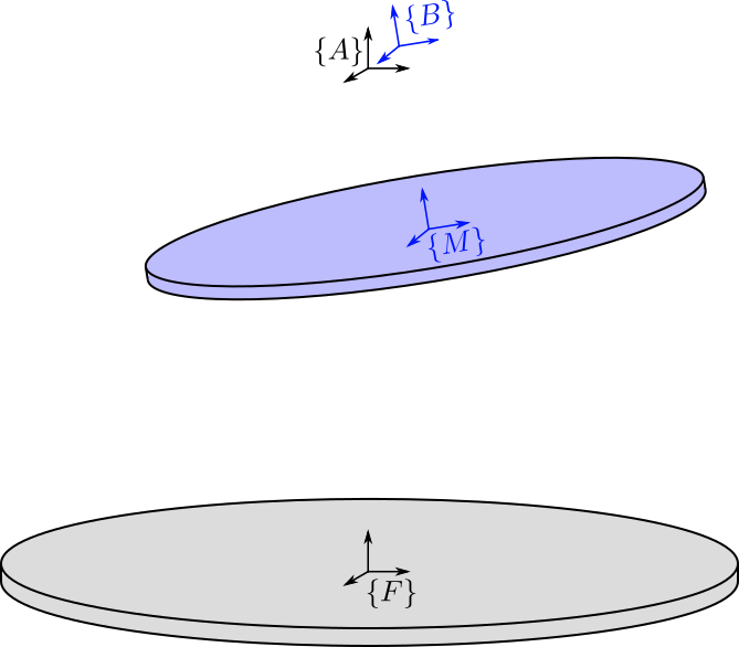
Figure 1: Definition of the Frames for the Stewart Platform

1.2 Location of the Spherical Joints

Then, we define the location of the spherical joints (see Figure 2):

\(\bm{a}_{i}\) are the position of the spherical joints fixed to the fixed base
\(\bm{b}_{i}\) are the position of the spherical joints fixed to the moving platform

The location of the joints will define the Geometry of the Stewart platform. Many characteristics of the platform depend on the location of the joints.

The location of the joints can be set to arbitrary positions or it can be computed to obtain specific configurations such as:

A cubic configuration: function generateCubicConfiguration (described in this file)
A symmetrical configuration

A function (generateGeneralConfiguration) to set the position of the joints on a circle is described here.

The location of the spherical joints are then given by \({}^{F}\bm{a}_{i}\) and \({}^{M}\bm{b}_{i}\).

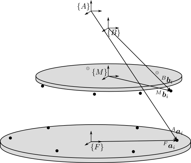
Figure 2: Position of the Spherical/Universal joints for the Stewart Platform

1.3 Length and orientation of the struts

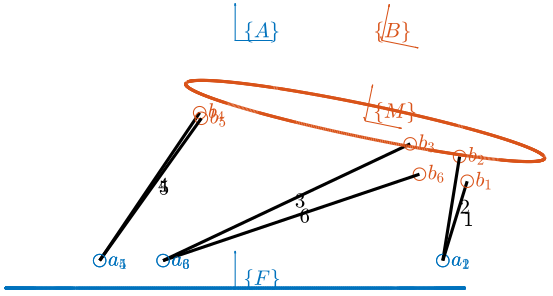
From the location of the joints (\({}^{F}\bm{a}_{i}\) and \({}^{M}\bm{b}_{i}\)), we compute the length \(l_i\) and orientation of each strut \(\hat{\bm{s}}_i\) (unit vector aligned with the strut). The length and orientation of each strut is represented in figure 3.

This is done with the computeJointsPose function (link).

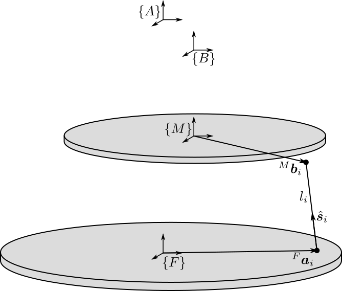
Figure 3: Length \(l_i\) and orientation \(\hat{\bm{s}}_i\) of the Stewart platform struts

1.4 Rest Position of the Stewart platform

We may want to initialize the Stewart platform in some position and orientation that corresponds to its rest position.

To do so, we choose:

the position of \(\bm{O}_B\) expressed in \(\{A\}\) using \({}^A\bm{P}\)
the orientation of \(\{B\}\) expressed in \(\{A\}\) using a rotation matrix \({}^{A}\bm{R}_{B}\)

Then, the function initializeStewartPose (link) compute the corresponding initial and rest position of each of the strut.

2 Definition of the Inertia and geometry of the Fixed base, Mobile platform and Struts

Now that the geometry of the Stewart platform has been defined, we have to choose the inertia of:

The Fixed base
The Mobile platform
The two parts of the struts

The inertia of these elements will modify the dynamics of the systems. It is thus important to set them properly.

2.1 Inertia and Geometry of the Fixed and Mobile platforms

In order to set the inertia of the fixed and mobile platforms, we can use the following function that assume that both platforms are cylindrical:

initializeCylindricalPlatforms (link): by choosing the height, radius and mass of the platforms, it computes the inertia matrix that will be used for simulation

2.2 Inertia and Geometry of the struts

Similarly for the struts, we suppose here that they have a cylindrical shape. They are initialize with the following function:

initializeCylindricalStruts (link): the two parts of each strut are supposed to by cylindrical. We can set the mass and geometry of both strut parts.

3 Definition of the stiffness and damping of the joints

The global stiffness and damping of the Stewart platform depends on its geometry but also on the stiffness and damping of:

the actuator because of the finite stiffness of the actuator / linear guide
the spherical joints

3.1 Stiffness and Damping of the Actuator

Each Actuator is modeled by 3 elements in parallel (Figure 4):

A spring with a stiffness \(k_{i}\)
A dashpot with a damping \(c_{i}\)
An ideal force actuator generating a force \(\tau_i\)

Figure 4: Model of the Stewart platform actuator

The initialization of the stiffness and damping properties of the actuators is done with the initializeStrutDynamics (link).

3.2 Stiffness and Damping of the Spherical Joints

Even though we often suppose that the spherical joint are perfect in the sense that we neglect its stiffness and damping, we can set some rotation stiffness and damping of each of the spherical/universal joints.

This is done with the initializeJointDynamics function (link).

4 Summary of the Initialization Procedure and Matlab Example

The procedure to define the Stewart platform is the following:

Define the initial position of frames \(\{A\}\), \(\{B\}\), \(\{F\}\) and \(\{M\}\). We do that using the initializeFramesPositions function. We have to specify the total height of the Stewart platform \(H\) and the position \({}^{M}\bm{O}_{B}\) of \(\{B\}\) with respect to \(\{M\}\).
Compute the positions of joints \({}^{F}\bm{a}_{i}\) and \({}^{M}\bm{b}_{i}\). We can do that using various methods depending on the wanted architecture:
- generateCubicConfiguration permits to generate a cubic configuration
Compute the position and orientation of the joints with respect to the fixed base and the moving platform. This is done with the computeJointsPose function. If wanted, compute the rest position of each strut to have the wanted pose of the mobile platform with the function initializeStewartPose.
Define the mass and inertia of each element of the Stewart platform with the initializeCylindricalPlatforms and initializeCylindricalStruts
Define the dynamical properties of the Stewart platform by setting the stiffness and damping of the actuators and joints.

By following this procedure, we obtain a Matlab structure stewart that contains all the information for the Simscape model and for further analysis.

4.1 Example of the initialization of a Stewart Platform

Let’s first define the Stewart Platform Geometry.

stewart = initializeStewartPlatform();
stewart = initializeFramesPositions(stewart, 'H', 90e-3, 'MO_B', 45e-3);
stewart = generateGeneralConfiguration(stewart);
stewart = computeJointsPose(stewart);
stewart = initializeStewartPose(stewart, 'AP', [0;0;0], 'ARB', eye(3));

Then, define the inertia and geometry of the fixed base, mobile platform and struts.

stewart = initializeCylindricalPlatforms(stewart);
stewart = initializeCylindricalStruts(stewart);

We initialize the strut stiffness and damping properties.

stewart = initializeStrutDynamics(stewart, 'K', 1e6*ones(6,1), 'C', 1e2*ones(6,1));
stewart = initializeAmplifiedStrutDynamics(stewart);
stewart = initializeJointDynamics(stewart);

And finally the inertial sensors included in each strut.

stewart = initializeInertialSensor(stewart, 'type', 'none');

The obtained stewart Matlab structure contains all the information for analysis of the Stewart platform and for simulations using Simscape.

The function displayArchitecture can be used to display the current Stewart configuration:

displayArchitecture(stewart, 'views', 'all');

Figure 5: Display of the current Stewart platform architecture (png, pdf)

There are many options to show or hides elements such as labels and frames. The documentation of the function is available here.

Let’s now move a little bit the top platform and re-display the configuration:

tx = 0.1; % [rad]
ty = 0.2; % [rad]
tz = 0.05; % [rad]

Rx = [1 0        0;
      0 cos(tx) -sin(tx);
      0 sin(tx)  cos(tx)];

Ry = [ cos(ty) 0 sin(ty);
      0        1 0;
      -sin(ty) 0 cos(ty)];

Rz = [cos(tz) -sin(tz) 0;
      sin(tz)  cos(tz) 0;
      0        0       1];

ARB = Rz*Ry*Rx;
AP = [0.08; 0; 0]; % [m]

displayArchitecture(stewart, 'AP', AP, 'ARB', ARB);
view([0 -1 0]);

Figure 6: Display of the Stewart platform architecture at some defined pose (png, pdf)

One can also use the describeStewartPlatform function to have a description of the current Stewart platform’s state.

describeStewartPlatform(stewart)
GEOMETRY:
- The height between the fixed based and the top platform is 90 [mm].
- Frame {A} is located 45 [mm] above the top platform.
- The initial length of the struts are:
	 95.2, 95.2, 95.2, 95.2, 95.2, 95.2 [mm]

ACTUATORS:
- The actuators are mechanicaly amplified.
- The vertical stiffness and damping contribution of the piezoelectric stack is:
	 ka = 2e+07 [N/m] 	 ca = 1e+01 [N/(m/s)]
- Vertical stiffness when the piezoelectric stack is removed is:
	 kr = 5e+06 [N/m] 	 cr = 1e+01 [N/(m/s)]

JOINTS:
- The joints on the fixed based are universal joints
- The joints on the mobile based are spherical joints
- The position of the joints on the fixed based with respect to {F} are (in [mm]):
	  113 	 -20 	  15
	  113 	  20 	  15
	 -39.3 	  108 	  15
	 -73.9 	  88.1 	  15
	 -73.9 	 -88.1 	  15
	 -39.3 	 -108 	  15
- The position of the joints on the mobile based with respect to {M} are (in [mm]):
	  57.9 	 -68.9 	 -15
	  57.9 	  68.9 	 -15
	  30.8 	  84.6 	 -15
	 -88.6 	  15.6 	 -15
	 -88.6 	 -15.6 	 -15
	  30.8 	 -84.6 	 -15

KINEMATICS:
'org_babel_eoe'
ans =
    'org_babel_eoe'

5 Functions

5.1 `initializeStewartPlatform`: Initialize the Stewart Platform structure

This Matlab function is accessible here.

Documentation

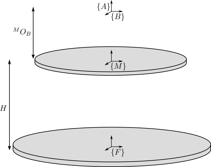
Figure 7: Definition of the position of the frames

Function description

function [stewart] = initializeStewartPlatform()
% initializeStewartPlatform - Initialize the stewart structure
%
% Syntax: [stewart] = initializeStewartPlatform(args)
%
% Outputs:
%    - stewart - A structure with the following sub-structures:
%      - platform_F -
%      - platform_M -
%      - joints_F   -
%      - joints_M   -
%      - struts_F   -
%      - struts_M   -
%      - actuators  -
%      - geometry   -
%      - properties -

Initialize the Stewart structure

stewart = struct();
stewart.platform_F = struct();
stewart.platform_M = struct();
stewart.joints_F   = struct();
stewart.joints_M   = struct();
stewart.struts_F   = struct();
stewart.struts_M   = struct();
stewart.actuators  = struct();
stewart.sensors    = struct();
stewart.sensors.inertial = struct();
stewart.sensors.force    = struct();
stewart.sensors.relative = struct();
stewart.geometry   = struct();
stewart.kinematics = struct();

5.2 `initializeFramesPositions`: Initialize the positions of frames {A}, {B}, {F} and {M}

This Matlab function is accessible here.

Documentation

Figure 8: Definition of the position of the frames

Function description

function [stewart] = initializeFramesPositions(stewart, args)
% initializeFramesPositions - Initialize the positions of frames {A}, {B}, {F} and {M}
%
% Syntax: [stewart] = initializeFramesPositions(stewart, args)
%
% Inputs:
%    - args - Can have the following fields:
%        - H    [1x1] - Total Height of the Stewart Platform (height from {F} to {M}) [m]
%        - MO_B [1x1] - Height of the frame {B} with respect to {M} [m]
%
% Outputs:
%    - stewart - A structure with the following fields:
%        - geometry.H      [1x1] - Total Height of the Stewart Platform [m]
%        - geometry.FO_M   [3x1] - Position of {M} with respect to {F} [m]
%        - platform_M.MO_B [3x1] - Position of {B} with respect to {M} [m]
%        - platform_F.FO_A [3x1] - Position of {A} with respect to {F} [m]

Optional Parameters

arguments
    stewart
    args.H    (1,1) double {mustBeNumeric, mustBePositive} = 90e-3
    args.MO_B (1,1) double {mustBeNumeric} = 50e-3
end

Compute the position of each frame

H = args.H; % Total Height of the Stewart Platform [m]

FO_M = [0; 0; H]; % Position of {M} with respect to {F} [m]

MO_B = [0; 0; args.MO_B]; % Position of {B} with respect to {M} [m]

FO_A = MO_B + FO_M; % Position of {A} with respect to {F} [m]

Populate the `stewart` structure

stewart.geometry.H      = H;
stewart.geometry.FO_M   = FO_M;
stewart.platform_M.MO_B = MO_B;
stewart.platform_F.FO_A = FO_A;

5.3 `generateGeneralConfiguration`: Generate a Very General Configuration

This Matlab function is accessible here.

Documentation

Joints are positions on a circle centered with the Z axis of {F} and {M} and at a chosen distance from {F} and {M}. The radius of the circles can be chosen as well as the angles where the joints are located (see Figure 9).

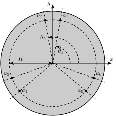
Figure 9: Position of the joints

Function description

function [stewart] = generateGeneralConfiguration(stewart, args)
% generateGeneralConfiguration - Generate a Very General Configuration
%
% Syntax: [stewart] = generateGeneralConfiguration(stewart, args)
%
% Inputs:
%    - args - Can have the following fields:
%        - FH  [1x1] - Height of the position of the fixed joints with respect to the frame {F} [m]
%        - FR  [1x1] - Radius of the position of the fixed joints in the X-Y [m]
%        - FTh [6x1] - Angles of the fixed joints in the X-Y plane with respect to the X axis [rad]
%        - MH  [1x1] - Height of the position of the mobile joints with respect to the frame {M} [m]
%        - FR  [1x1] - Radius of the position of the mobile joints in the X-Y [m]
%        - MTh [6x1] - Angles of the mobile joints in the X-Y plane with respect to the X axis [rad]
%
% Outputs:
%    - stewart - updated Stewart structure with the added fields:
%        - platform_F.Fa  [3x6] - Its i'th column is the position vector of joint ai with respect to {F}
%        - platform_M.Mb  [3x6] - Its i'th column is the position vector of joint bi with respect to {M}

Optional Parameters

arguments
    stewart
    args.FH  (1,1) double {mustBeNumeric, mustBePositive} = 15e-3
    args.FR  (1,1) double {mustBeNumeric, mustBePositive} = 115e-3;
    args.FTh (6,1) double {mustBeNumeric} = [-10, 10, 120-10, 120+10, 240-10, 240+10]*(pi/180);
    args.MH  (1,1) double {mustBeNumeric, mustBePositive} = 15e-3
    args.MR  (1,1) double {mustBeNumeric, mustBePositive} = 90e-3;
    args.MTh (6,1) double {mustBeNumeric} = [-60+10, 60-10, 60+10, 180-10, 180+10, -60-10]*(pi/180);
end

Compute the pose

Fa = zeros(3,6);
Mb = zeros(3,6);

for i = 1:6
  Fa(:,i) = [args.FR*cos(args.FTh(i)); args.FR*sin(args.FTh(i));  args.FH];
  Mb(:,i) = [args.MR*cos(args.MTh(i)); args.MR*sin(args.MTh(i)); -args.MH];
end

Populate the `stewart` structure

stewart.platform_F.Fa = Fa;
stewart.platform_M.Mb = Mb;

5.4 `computeJointsPose`: Compute the Pose of the Joints

This Matlab function is accessible here.

Documentation

Figure 10: Position and orientation of the struts

Function description

function [stewart] = computeJointsPose(stewart, args)
% computeJointsPose -
%
% Syntax: [stewart] = computeJointsPose(stewart, args)
%
% Inputs:
%    - stewart - A structure with the following fields
%        - platform_F.Fa   [3x6] - Its i'th column is the position vector of joint ai with respect to {F}
%        - platform_M.Mb   [3x6] - Its i'th column is the position vector of joint bi with respect to {M}
%        - platform_F.FO_A [3x1] - Position of {A} with respect to {F}
%        - platform_M.MO_B [3x1] - Position of {B} with respect to {M}
%        - geometry.FO_M   [3x1] - Position of {M} with respect to {F}
%    - args - Can have the following fields:
%        - AP   [3x1] - The wanted position of {B} with respect to {A}
%        - ARB  [3x3] - The rotation matrix that gives the wanted orientation of {B} with respect to {A}
%
% Outputs:
%    - stewart - A structure with the following added fields
%        - geometry.Aa    [3x6]   - The i'th column is the position of ai with respect to {A}
%        - geometry.Ab    [3x6]   - The i'th column is the position of bi with respect to {A}
%        - geometry.Ba    [3x6]   - The i'th column is the position of ai with respect to {B}
%        - geometry.Bb    [3x6]   - The i'th column is the position of bi with respect to {B}
%        - geometry.l     [6x1]   - The i'th element is the initial length of strut i
%        - geometry.As    [3x6]   - The i'th column is the unit vector of strut i expressed in {A}
%        - geometry.Bs    [3x6]   - The i'th column is the unit vector of strut i expressed in {B}
%        - struts_F.l     [6x1]   - Length of the Fixed part of the i'th strut
%        - struts_M.l     [6x1]   - Length of the Mobile part of the i'th strut
%        - platform_F.FRa [3x3x6] - The i'th 3x3 array is the rotation matrix to orientate the bottom of the i'th strut from {F}
%        - platform_M.MRb [3x3x6] - The i'th 3x3 array is the rotation matrix to orientate the top of the i'th strut from {M}

Optional Parameters

arguments
    stewart
    args.AP  (3,1) double {mustBeNumeric} = zeros(3,1)
    args.ARB (3,3) double {mustBeNumeric} = eye(3)
end

Check the `stewart` structure elements

assert(isfield(stewart.platform_F, 'Fa'),   'stewart.platform_F should have attribute Fa')
Fa = stewart.platform_F.Fa;

assert(isfield(stewart.platform_M, 'Mb'),   'stewart.platform_M should have attribute Mb')
Mb = stewart.platform_M.Mb;

assert(isfield(stewart.platform_F, 'FO_A'), 'stewart.platform_F should have attribute FO_A')
FO_A = stewart.platform_F.FO_A;

assert(isfield(stewart.platform_M, 'MO_B'), 'stewart.platform_M should have attribute MO_B')
MO_B = stewart.platform_M.MO_B;

assert(isfield(stewart.geometry,   'FO_M'), 'stewart.geometry should have attribute FO_M')
FO_M = stewart.geometry.FO_M;

Compute the position of the Joints

Aa = Fa - repmat(FO_A, [1, 6]);
Bb = Mb - repmat(MO_B, [1, 6]);

Original:

Ab = Bb - repmat(-MO_B-FO_M+FO_A, [1, 6]);
Ba = Aa - repmat( MO_B+FO_M-FO_A, [1, 6]);

Translation & Rotation: (Rotation and then translation)

Ab = args.ARB *Bb - repmat(-args.AP, [1, 6]);
Ba = args.ARB'*Aa - repmat( args.AP, [1, 6]);

Compute the strut length and orientation

As = (Ab - Aa)./vecnorm(Ab - Aa); % As_i is the i'th vector of As

l = vecnorm(Ab - Aa)';

Bs = (Bb - Ba)./vecnorm(Bb - Ba);

Compute the orientation of the Joints

FRa = zeros(3,3,6);
MRb = zeros(3,3,6);

for i = 1:6
  FRa(:,:,i) = [cross([0;1;0], As(:,i)) , cross(As(:,i), cross([0;1;0], As(:,i))) , As(:,i)];
  FRa(:,:,i) = FRa(:,:,i)./vecnorm(FRa(:,:,i));

  MRb(:,:,i) = [cross([0;1;0], Bs(:,i)) , cross(Bs(:,i), cross([0;1;0], Bs(:,i))) , Bs(:,i)];
  MRb(:,:,i) = MRb(:,:,i)./vecnorm(MRb(:,:,i));
end

Populate the `stewart` structure

stewart.geometry.Aa = Aa;
stewart.geometry.Ab = Ab;
stewart.geometry.Ba = Ba;
stewart.geometry.Bb = Bb;
stewart.geometry.As = As;
stewart.geometry.Bs = Bs;
stewart.geometry.l  = l;

stewart.struts_F.l  = l/2;
stewart.struts_M.l  = l/2;

stewart.platform_F.FRa = FRa;
stewart.platform_M.MRb = MRb;

5.5 `initializeStewartPose`: Determine the initial stroke in each leg to have the wanted pose

This Matlab function is accessible here.

Function description

function [stewart] = initializeStewartPose(stewart, args)
% initializeStewartPose - Determine the initial stroke in each leg to have the wanted pose
%                         It uses the inverse kinematic
%
% Syntax: [stewart] = initializeStewartPose(stewart, args)
%
% Inputs:
%    - stewart - A structure with the following fields
%        - Aa   [3x6] - The positions ai expressed in {A}
%        - Bb   [3x6] - The positions bi expressed in {B}
%    - args - Can have the following fields:
%        - AP   [3x1] - The wanted position of {B} with respect to {A}
%        - ARB  [3x3] - The rotation matrix that gives the wanted orientation of {B} with respect to {A}
%
% Outputs:
%    - stewart - updated Stewart structure with the added fields:
%      - actuators.Leq [6x1] - The 6 needed displacement of the struts from the initial position in [m] to have the wanted pose of {B} w.r.t. {A}

Optional Parameters

arguments
    stewart
    args.AP  (3,1) double {mustBeNumeric} = zeros(3,1)
    args.ARB (3,3) double {mustBeNumeric} = eye(3)
end

Use the Inverse Kinematic function

[Li, dLi] = inverseKinematics(stewart, 'AP', args.AP, 'ARB', args.ARB);

Populate the `stewart` structure

stewart.actuators.Leq = dLi;

5.6 `initializeCylindricalPlatforms`: Initialize the geometry of the Fixed and Mobile Platforms

This Matlab function is accessible here.

Function description

function [stewart] = initializeCylindricalPlatforms(stewart, args)
% initializeCylindricalPlatforms - Initialize the geometry of the Fixed and Mobile Platforms
%
% Syntax: [stewart] = initializeCylindricalPlatforms(args)
%
% Inputs:
%    - args - Structure with the following fields:
%        - Fpm [1x1] - Fixed Platform Mass [kg]
%        - Fph [1x1] - Fixed Platform Height [m]
%        - Fpr [1x1] - Fixed Platform Radius [m]
%        - Mpm [1x1] - Mobile Platform Mass [kg]
%        - Mph [1x1] - Mobile Platform Height [m]
%        - Mpr [1x1] - Mobile Platform Radius [m]
%
% Outputs:
%    - stewart - updated Stewart structure with the added fields:
%      - platform_F [struct] - structure with the following fields:
%        - type = 1
%        - M [1x1] - Fixed Platform Mass [kg]
%        - I [3x3] - Fixed Platform Inertia matrix [kg*m^2]
%        - H [1x1] - Fixed Platform Height [m]
%        - R [1x1] - Fixed Platform Radius [m]
%      - platform_M [struct] - structure with the following fields:
%        - M [1x1] - Mobile Platform Mass [kg]
%        - I [3x3] - Mobile Platform Inertia matrix [kg*m^2]
%        - H [1x1] - Mobile Platform Height [m]
%        - R [1x1] - Mobile Platform Radius [m]

Optional Parameters

arguments
    stewart
    args.Fpm (1,1) double {mustBeNumeric, mustBePositive} = 1
    args.Fph (1,1) double {mustBeNumeric, mustBePositive} = 10e-3
    args.Fpr (1,1) double {mustBeNumeric, mustBePositive} = 125e-3
    args.Mpm (1,1) double {mustBeNumeric, mustBePositive} = 1
    args.Mph (1,1) double {mustBeNumeric, mustBePositive} = 10e-3
    args.Mpr (1,1) double {mustBeNumeric, mustBePositive} = 100e-3
end

Compute the Inertia matrices of platforms

I_F = diag([1/12*args.Fpm * (3*args.Fpr^2 + args.Fph^2), ...
            1/12*args.Fpm * (3*args.Fpr^2 + args.Fph^2), ...
            1/2 *args.Fpm * args.Fpr^2]);

I_M = diag([1/12*args.Mpm * (3*args.Mpr^2 + args.Mph^2), ...
            1/12*args.Mpm * (3*args.Mpr^2 + args.Mph^2), ...
            1/2 *args.Mpm * args.Mpr^2]);

Populate the `stewart` structure

stewart.platform_F.type = 1;

stewart.platform_F.I = I_F;
stewart.platform_F.M = args.Fpm;
stewart.platform_F.R = args.Fpr;
stewart.platform_F.H = args.Fph;

stewart.platform_M.type = 1;

stewart.platform_M.I = I_M;
stewart.platform_M.M = args.Mpm;
stewart.platform_M.R = args.Mpr;
stewart.platform_M.H = args.Mph;

5.7 `initializeCylindricalStruts`: Define the inertia of cylindrical struts

This Matlab function is accessible here.

Function description

function [stewart] = initializeCylindricalStruts(stewart, args)
% initializeCylindricalStruts - Define the mass and moment of inertia of cylindrical struts
%
% Syntax: [stewart] = initializeCylindricalStruts(args)
%
% Inputs:
%    - args - Structure with the following fields:
%        - Fsm [1x1] - Mass of the Fixed part of the struts [kg]
%        - Fsh [1x1] - Height of cylinder for the Fixed part of the struts [m]
%        - Fsr [1x1] - Radius of cylinder for the Fixed part of the struts [m]
%        - Msm [1x1] - Mass of the Mobile part of the struts [kg]
%        - Msh [1x1] - Height of cylinder for the Mobile part of the struts [m]
%        - Msr [1x1] - Radius of cylinder for the Mobile part of the struts [m]
%
% Outputs:
%    - stewart - updated Stewart structure with the added fields:
%      - struts_F [struct] - structure with the following fields:
%        - M [6x1]   - Mass of the Fixed part of the struts [kg]
%        - I [3x3x6] - Moment of Inertia for the Fixed part of the struts [kg*m^2]
%        - H [6x1]   - Height of cylinder for the Fixed part of the struts [m]
%        - R [6x1]   - Radius of cylinder for the Fixed part of the struts [m]
%      - struts_M [struct] - structure with the following fields:
%        - M [6x1]   - Mass of the Mobile part of the struts [kg]
%        - I [3x3x6] - Moment of Inertia for the Mobile part of the struts [kg*m^2]
%        - H [6x1]   - Height of cylinder for the Mobile part of the struts [m]
%        - R [6x1]   - Radius of cylinder for the Mobile part of the struts [m]

Optional Parameters

arguments
    stewart
    args.type_F    char   {mustBeMember(args.type_F,{'cylindrical', 'none'})} = 'cylindrical'
    args.type_M    char   {mustBeMember(args.type_M,{'cylindrical', 'none'})} = 'cylindrical'
    args.Fsm (1,1) double {mustBeNumeric, mustBePositive} = 0.1
    args.Fsh (1,1) double {mustBeNumeric, mustBePositive} = 50e-3
    args.Fsr (1,1) double {mustBeNumeric, mustBePositive} = 5e-3
    args.Msm (1,1) double {mustBeNumeric, mustBePositive} = 0.1
    args.Msh (1,1) double {mustBeNumeric, mustBePositive} = 50e-3
    args.Msr (1,1) double {mustBeNumeric, mustBePositive} = 5e-3
end

Compute the properties of the cylindrical struts

Fsm = ones(6,1).*args.Fsm;
Fsh = ones(6,1).*args.Fsh;
Fsr = ones(6,1).*args.Fsr;

Msm = ones(6,1).*args.Msm;
Msh = ones(6,1).*args.Msh;
Msr = ones(6,1).*args.Msr;

I_F = zeros(3, 3, 6); % Inertia of the "fixed" part of the strut
I_M = zeros(3, 3, 6); % Inertia of the "mobile" part of the strut

for i = 1:6
  I_F(:,:,i) = diag([1/12 * Fsm(i) * (3*Fsr(i)^2 + Fsh(i)^2), ...
                     1/12 * Fsm(i) * (3*Fsr(i)^2 + Fsh(i)^2), ...
                     1/2  * Fsm(i) * Fsr(i)^2]);

  I_M(:,:,i) = diag([1/12 * Msm(i) * (3*Msr(i)^2 + Msh(i)^2), ...
                     1/12 * Msm(i) * (3*Msr(i)^2 + Msh(i)^2), ...
                     1/2  * Msm(i) * Msr(i)^2]);
end

Populate the `stewart` structure

switch args.type_M
  case 'cylindrical'
    stewart.struts_M.type = 1;
  case 'none'
    stewart.struts_M.type = 2;
end

stewart.struts_M.I = I_M;
stewart.struts_M.M = Msm;
stewart.struts_M.R = Msr;
stewart.struts_M.H = Msh;

switch args.type_F
  case 'cylindrical'
    stewart.struts_F.type = 1;
  case 'none'
    stewart.struts_F.type = 2;
end

stewart.struts_F.I = I_F;
stewart.struts_F.M = Fsm;
stewart.struts_F.R = Fsr;
stewart.struts_F.H = Fsh;

5.8 `initializeStrutDynamics`: Add Stiffness and Damping properties of each strut

This Matlab function is accessible here.

Documentation

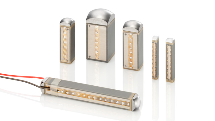
Figure 11: Example of a piezoelectric stach actuator (PI)

A simplistic model of such amplified actuator is shown in Figure 12 where:

\(K\) represent the vertical stiffness of the actuator
\(C\) represent the vertical damping of the actuator
\(F\) represents the force applied by the actuator
\(F_{m}\) represents the total measured force
\(v_{m}\) represents the absolute velocity of the top part of the actuator
\(d_{m}\) represents the total relative displacement of the actuator

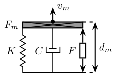
Figure 12: Simple model of an Actuator

Function description

function [stewart] = initializeStrutDynamics(stewart, args)
% initializeStrutDynamics - Add Stiffness and Damping properties of each strut
%
% Syntax: [stewart] = initializeStrutDynamics(args)
%
% Inputs:
%    - args - Structure with the following fields:
%        - K [6x1] - Stiffness of each strut [N/m]
%        - C [6x1] - Damping of each strut [N/(m/s)]
%
% Outputs:
%    - stewart - updated Stewart structure with the added fields:
%      - actuators.type = 1
%      - actuators.K [6x1] - Stiffness of each strut [N/m]
%      - actuators.C [6x1] - Damping of each strut [N/(m/s)]

Optional Parameters

arguments
    stewart
    args.K (6,1) double {mustBeNumeric, mustBeNonnegative} = 20e6*ones(6,1)
    args.C (6,1) double {mustBeNumeric, mustBeNonnegative} = 2e1*ones(6,1)
end

Add Stiffness and Damping properties of each strut

stewart.actuators.type = 1;

stewart.actuators.K = args.K;
stewart.actuators.C = args.C;

5.9 `initializeAmplifiedStrutDynamics`: Add Stiffness and Damping properties of each strut for an amplified piezoelectric actuator

This Matlab function is accessible here.

Documentation

An amplified piezoelectric actuator is shown in Figure 13.

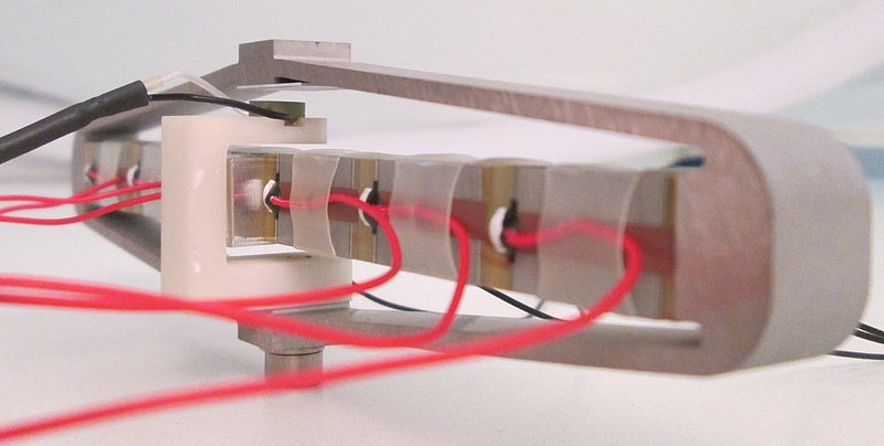
Figure 13: Example of an Amplified piezoelectric actuator with an integrated displacement sensor (Cedrat Technologies)

A simplistic model of such amplified actuator is shown in Figure 14 where the parameters are described in Table 1.

Table 1: Parameters used for the model of the APA 100M
	Meaning
\(k_e\)	Stiffness used to adjust the pole of the isolator
\(k_1\)	Stiffness of the metallic suspension when the stack is removed
\(k_a\)	Stiffness of the actuator
\(c_1\)	Added viscous damping

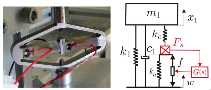
Figure 14: Picture of an APA100M from Cedrat Technologies. Simplified model of a one DoF payload mounted on such isolator

Function description

function [stewart] = initializeAmplifiedStrutDynamics(stewart, args)
% initializeAmplifiedStrutDynamics - Add Stiffness and Damping properties of each strut
%
% Syntax: [stewart] = initializeAmplifiedStrutDynamics(args)
%
% Inputs:
%    - args - Structure with the following fields:
%        - Ka [6x1] - Stiffness of the actuator [N/m]
%        - Ke [6x1] - Stiffness used to adjust the pole of the isolator [N/m]
%        - K1 [6x1] - Stiffness of the metallic suspension when the stack is removed [N/m]
%        - C1 [6x1] - Added viscous damping [N/(m/s)]
%
% Outputs:
%    - stewart - updated Stewart structure with the added fields:
%      - actuators.type = 2
%      - actuators.K   [6x1] - Total Stiffness of each strut [N/m]
%      - actuators.C   [6x1] - Total Damping of each strut [N/(m/s)]
%      - actuators.Ka [6x1] - Stiffness of the actuator [N/m]
%      - actuators.Ke [6x1] - Stiffness used to adjust the pole of the isolator [N/m]
%      - actuators.K1 [6x1] - Stiffness of the metallic suspension when the stack is removed [N/m]
%      - actuators.C1 [6x1] - Added viscous damping [N/(m/s)]

Optional Parameters

arguments
    stewart
    args.Ke (6,1) double {mustBeNumeric, mustBeNonnegative} = 1.5e6*ones(6,1)
    args.Ka (6,1) double {mustBeNumeric, mustBeNonnegative} = 43e6*ones(6,1)
    args.K1 (6,1) double {mustBeNumeric, mustBeNonnegative} = 0.4e6*ones(6,1)
    args.C1 (6,1) double {mustBeNumeric, mustBeNonnegative} = 10*ones(6,1)
end

Compute the total stiffness and damping

K = args.K1 + args.Ka.*args.Ke./(args.Ka + args.Ke);
C = args.C1;

Populate the `stewart` structure

stewart.actuators.type = 2;

stewart.actuators.Ka = args.Ka;
stewart.actuators.Ke = args.Ke;
stewart.actuators.K1 = args.K1;
stewart.actuators.C1 = args.C1;

stewart.actuators.K = K;
stewart.actuators.C = C;

5.10 `initializeFlexibleStrutDynamics`: Model each strut with a flexible element

This Matlab function is accessible here.

Function description

function [stewart] = initializeFlexibleStrutDynamics(stewart, args)
% initializeFlexibleStrutDynamics - Add Stiffness and Damping properties of each strut
%
% Syntax: [stewart] = initializeFlexibleStrutDynamics(args)
%
% Inputs:
%    - args - Structure with the following fields:
%        - K [nxn] - Vertical stiffness contribution of the piezoelectric stack [N/m]
%        - M [nxn] - Vertical damping contribution of the piezoelectric stack [N/(m/s)]
%        - xi        [1x1] - Vertical (residual) stiffness when the piezoelectric stack is removed [N/m]
%        - step_file [6x1] - Vertical (residual) damping when the piezoelectric stack is removed [N/(m/s)]
%        - Gf [6x1] - Gain from strain in [m] to measured [N] such that it matches
%
% Outputs:
%    - stewart - updated Stewart structure with the added fields:

Optional Parameters

arguments
    stewart
    args.K        double {mustBeNumeric} = zeros(6,6)
    args.M        double {mustBeNumeric} = zeros(6,6)
    args.H        double {mustBeNumeric} = 0
    args.n_xyz    double {mustBeNumeric} = zeros(2,3)
    args.xi       double {mustBeNumeric} = 0.1
    args.Gf       double {mustBeNumeric} = 1
    args.step_file char {} = ''
end

Compute the axial offset

stewart.actuators.ax_off = (stewart.geometry.l(1) - args.H)/2; % Axial Offset at the ends of the actuator

Populate the `stewart` structure

stewart.actuators.type = 3;

stewart.actuators.Km = args.K;
stewart.actuators.Mm = args.M;

stewart.actuators.n_xyz = args.n_xyz;
stewart.actuators.xi = args.xi;

stewart.actuators.step_file = args.step_file;

stewart.actuators.K = args.K(3,3); % Axial Stiffness

stewart.actuators.Gf = args.Gf;

5.11 `initializeJointDynamics`: Add Stiffness and Damping properties for spherical joints

This Matlab function is accessible here.

Function description

function [stewart] = initializeJointDynamics(stewart, args)
% initializeJointDynamics - Add Stiffness and Damping properties for the spherical joints
%
% Syntax: [stewart] = initializeJointDynamics(args)
%
% Inputs:
%    - args - Structure with the following fields:
%        - type_F - 'universal', 'spherical', 'universal_p', 'spherical_p'
%        - type_M - 'universal', 'spherical', 'universal_p', 'spherical_p'
%        - Kf_M [6x1] - Bending (Rx, Ry) Stiffness for each top joints [(N.m)/rad]
%        - Kt_M [6x1] - Torsion (Rz) Stiffness for each top joints [(N.m)/rad]
%        - Cf_M [6x1] - Bending (Rx, Ry) Damping of each top joint [(N.m)/(rad/s)]
%        - Ct_M [6x1] - Torsion (Rz) Damping of each top joint [(N.m)/(rad/s)]
%        - Kf_F [6x1] - Bending (Rx, Ry) Stiffness for each bottom joints [(N.m)/rad]
%        - Kt_F [6x1] - Torsion (Rz) Stiffness for each bottom joints [(N.m)/rad]
%        - Cf_F [6x1] - Bending (Rx, Ry) Damping of each bottom joint [(N.m)/(rad/s)]
%        - Cf_F [6x1] - Torsion (Rz) Damping of each bottom joint [(N.m)/(rad/s)]
%
% Outputs:
%    - stewart - updated Stewart structure with the added fields:
%      - stewart.joints_F and stewart.joints_M:
%        - type - 1 (universal), 2 (spherical), 3 (universal perfect), 4 (spherical perfect)
%        - Kx, Ky, Kz [6x1] - Translation (Tx, Ty, Tz) Stiffness [N/m]
%        - Kf [6x1] - Flexion (Rx, Ry) Stiffness [(N.m)/rad]
%        - Kt [6x1] - Torsion (Rz) Stiffness [(N.m)/rad]
%        - Cx, Cy, Cz [6x1] - Translation (Rx, Ry) Damping [N/(m/s)]
%        - Cf [6x1] - Flexion (Rx, Ry) Damping [(N.m)/(rad/s)]
%        - Cb [6x1] - Torsion (Rz) Damping [(N.m)/(rad/s)]

Optional Parameters

arguments
    stewart
    args.type_F     char   {mustBeMember(args.type_F,{'universal', 'spherical', 'universal_p', 'spherical_p', 'universal_3dof', 'spherical_3dof', 'flexible'})} = 'universal'
    args.type_M     char   {mustBeMember(args.type_M,{'universal', 'spherical', 'universal_p', 'spherical_p', 'universal_3dof', 'spherical_3dof', 'flexible'})} = 'spherical'
    args.Kf_M (6,1) double {mustBeNumeric, mustBeNonnegative} = 33*ones(6,1)
    args.Cf_M (6,1) double {mustBeNumeric, mustBeNonnegative} = 1e-4*ones(6,1)
    args.Kt_M (6,1) double {mustBeNumeric, mustBeNonnegative} = 236*ones(6,1)
    args.Ct_M (6,1) double {mustBeNumeric, mustBeNonnegative} = 1e-3*ones(6,1)
    args.Kf_F (6,1) double {mustBeNumeric, mustBeNonnegative} = 33*ones(6,1)
    args.Cf_F (6,1) double {mustBeNumeric, mustBeNonnegative} = 1e-4*ones(6,1)
    args.Kt_F (6,1) double {mustBeNumeric, mustBeNonnegative} = 236*ones(6,1)
    args.Ct_F (6,1) double {mustBeNumeric, mustBeNonnegative} = 1e-3*ones(6,1)
    args.Ka_F (6,1) double {mustBeNumeric, mustBeNonnegative} = 1.2e8*ones(6,1)
    args.Ca_F (6,1) double {mustBeNumeric, mustBeNonnegative} = 1e1*ones(6,1)
    args.Kr_F (6,1) double {mustBeNumeric, mustBeNonnegative} = 1.1e7*ones(6,1)
    args.Cr_F (6,1) double {mustBeNumeric, mustBeNonnegative} = 1e1*ones(6,1)
    args.Ka_M (6,1) double {mustBeNumeric, mustBeNonnegative} = 1.2e8*ones(6,1)
    args.Ca_M (6,1) double {mustBeNumeric, mustBeNonnegative} = 1e1*ones(6,1)
    args.Kr_M (6,1) double {mustBeNumeric, mustBeNonnegative} = 1.1e7*ones(6,1)
    args.Cr_M (6,1) double {mustBeNumeric, mustBeNonnegative} = 1e1*ones(6,1)
    args.K_M        double {mustBeNumeric} = zeros(6,6)
    args.M_M        double {mustBeNumeric} = zeros(6,6)
    args.n_xyz_M    double {mustBeNumeric} = zeros(2,3)
    args.xi_M       double {mustBeNumeric} = 0.1
    args.step_file_M char {} = ''
    args.K_F        double {mustBeNumeric} = zeros(6,6)
    args.M_F        double {mustBeNumeric} = zeros(6,6)
    args.n_xyz_F    double {mustBeNumeric} = zeros(2,3)
    args.xi_F       double {mustBeNumeric} = 0.1
    args.step_file_F char {} = ''
end

Add Actuator Type

switch args.type_F
  case 'universal'
    stewart.joints_F.type = 1;
  case 'spherical'
    stewart.joints_F.type = 2;
  case 'universal_p'
    stewart.joints_F.type = 3;
  case 'spherical_p'
    stewart.joints_F.type = 4;
  case 'flexible'
    stewart.joints_F.type = 5;
  case 'universal_3dof'
    stewart.joints_F.type = 6;
  case 'spherical_3dof'
    stewart.joints_F.type = 7;
end

switch args.type_M
  case 'universal'
    stewart.joints_M.type = 1;
  case 'spherical'
    stewart.joints_M.type = 2;
  case 'universal_p'
    stewart.joints_M.type = 3;
  case 'spherical_p'
    stewart.joints_M.type = 4;
  case 'flexible'
    stewart.joints_M.type = 5;
  case 'universal_3dof'
    stewart.joints_M.type = 6;
  case 'spherical_3dof'
    stewart.joints_M.type = 7;
end

Add Stiffness and Damping in Translation of each strut

Axial and Radial (shear) Stiffness

stewart.joints_M.Ka = args.Ka_M;
stewart.joints_M.Kr = args.Kr_M;

stewart.joints_F.Ka = args.Ka_F;
stewart.joints_F.Kr = args.Kr_F;

Translation Damping

stewart.joints_M.Ca = args.Ca_M;
stewart.joints_M.Cr = args.Cr_M;

stewart.joints_F.Ca = args.Ca_F;
stewart.joints_F.Cr = args.Cr_F;

Add Stiffness and Damping in Rotation of each strut

Rotational Stiffness

stewart.joints_M.Kf = args.Kf_M;
stewart.joints_M.Kt = args.Kt_M;

stewart.joints_F.Kf = args.Kf_F;
stewart.joints_F.Kt = args.Kt_F;

Rotational Damping

stewart.joints_M.Cf = args.Cf_M;
stewart.joints_M.Ct = args.Ct_M;

stewart.joints_F.Cf = args.Cf_F;
stewart.joints_F.Ct = args.Ct_F;

Stiffness and Mass matrices for flexible joint

stewart.joints_F.M = args.M_F;
stewart.joints_F.K = args.K_F;
stewart.joints_F.n_xyz = args.n_xyz_F;
stewart.joints_F.xi = args.xi_F;
stewart.joints_F.xi = args.xi_F;
stewart.joints_F.step_file = args.step_file_F;

stewart.joints_M.M = args.M_M;
stewart.joints_M.K = args.K_M;
stewart.joints_M.n_xyz = args.n_xyz_M;
stewart.joints_M.xi = args.xi_M;
stewart.joints_M.step_file = args.step_file_M;

5.12 `initializeInertialSensor`: Initialize the inertial sensor in each strut

This Matlab function is accessible here.

Geophone - Working Principle

From the schematic of the Z-axis geophone shown in Figure 15, we can write the transfer function from the support velocity \(\dot{w}\) to the relative velocity of the inertial mass \(\dot{d}\): \[ \frac{\dot{d}}{\dot{w}} = \frac{-\frac{s^2}{{\omega_0}^2}}{\frac{s^2}{{\omega_0}^2} + 2 \xi \frac{s}{\omega_0} + 1} \] with:

\(\omega_0 = \sqrt{\frac{k}{m}}\)
\(\xi = \frac{1}{2} \sqrt{\frac{m}{k}}\)

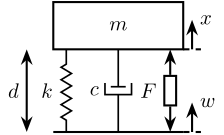
Figure 15: Schematic of a Z-Axis geophone

We see that at frequencies above \(\omega_0\): \[ \frac{\dot{d}}{\dot{w}} \approx -1 \]

And thus, the measurement of the relative velocity of the mass with respect to its support gives the absolute velocity of the support.

We generally want to have the smallest resonant frequency \(\omega_0\) to measure low frequency absolute velocity, however there is a trade-off between \(\omega_0\) and the mass of the inertial mass.

Accelerometer - Working Principle

From the schematic of the Z-axis accelerometer shown in Figure 16, we can write the transfer function from the support acceleration \(\ddot{w}\) to the relative position of the inertial mass \(d\): \[ \frac{d}{\ddot{w}} = \frac{-\frac{1}{{\omega_0}^2}}{\frac{s^2}{{\omega_0}^2} + 2 \xi \frac{s}{\omega_0} + 1} \] with:

\(\omega_0 = \sqrt{\frac{k}{m}}\)
\(\xi = \frac{1}{2} \sqrt{\frac{m}{k}}\)

Figure 16: Schematic of a Z-Axis geophone

We see that at frequencies below \(\omega_0\): \[ \frac{d}{\ddot{w}} \approx -\frac{1}{{\omega_0}^2} \]

And thus, the measurement of the relative displacement of the mass with respect to its support gives the absolute acceleration of the support.

Note that there is trade-off between:

the highest measurable acceleration \(\omega_0\)
the sensitivity of the accelerometer which is equal to \(-\frac{1}{{\omega_0}^2}\)

Function description

function [stewart] = initializeInertialSensor(stewart, args)
% initializeInertialSensor - Initialize the inertial sensor in each strut
%
% Syntax: [stewart] = initializeInertialSensor(args)
%
% Inputs:
%    - args - Structure with the following fields:
%        - type       - 'geophone', 'accelerometer', 'none'
%        - mass [1x1] - Weight of the inertial mass [kg]
%        - freq [1x1] - Cutoff frequency [Hz]
%
% Outputs:
%    - stewart - updated Stewart structure with the added fields:
%      - stewart.sensors.inertial
%        - type    - 1 (geophone), 2 (accelerometer), 3 (none)
%        - K [1x1] - Stiffness [N/m]
%        - C [1x1] - Damping [N/(m/s)]
%        - M [1x1] - Inertial Mass [kg]
%        - G [1x1] - Gain

Optional Parameters

arguments
    stewart
    args.type       char   {mustBeMember(args.type,{'geophone', 'accelerometer', 'none'})} = 'none'
    args.mass (1,1) double {mustBeNumeric, mustBeNonnegative} = 1e-2
    args.freq (1,1) double {mustBeNumeric, mustBeNonnegative} = 1e3
end

Compute the properties of the sensor

sensor = struct();

switch args.type
  case 'geophone'
    sensor.type = 1;

    sensor.M = args.mass;
    sensor.K = sensor.M * (2*pi*args.freq)^2;
    sensor.C = 2*sqrt(sensor.M * sensor.K);
  case 'accelerometer'
    sensor.type = 2;

    sensor.M = args.mass;
    sensor.K = sensor.M * (2*pi*args.freq)^2;
    sensor.C = 2*sqrt(sensor.M * sensor.K);
    sensor.G = -sensor.K/sensor.M;
  case 'none'
    sensor.type = 3;
end

Populate the `stewart` structure

stewart.sensors.inertial = sensor;

5.13 `displayArchitecture`: 3D plot of the Stewart platform architecture

This Matlab function is accessible here.

Function description

function [] = displayArchitecture(stewart, args)
% displayArchitecture - 3D plot of the Stewart platform architecture
%
% Syntax: [] = displayArchitecture(args)
%
% Inputs:
%    - stewart
%    - args - Structure with the following fields:
%        - AP   [3x1] - The wanted position of {B} with respect to {A}
%        - ARB  [3x3] - The rotation matrix that gives the wanted orientation of {B} with respect to {A}
%        - ARB  [3x3] - The rotation matrix that gives the wanted orientation of {B} with respect to {A}
%        - F_color [color] - Color used for the Fixed elements
%        - M_color [color] - Color used for the Mobile elements
%        - L_color [color] - Color used for the Legs elements
%        - frames    [true/false] - Display the Frames
%        - legs      [true/false] - Display the Legs
%        - joints    [true/false] - Display the Joints
%        - labels    [true/false] - Display the Labels
%        - platforms [true/false] - Display the Platforms
%        - views     ['all', 'xy', 'yz', 'xz', 'default'] -
%
% Outputs:

Optional Parameters

arguments
    stewart
    args.AP  (3,1) double {mustBeNumeric} = zeros(3,1)
    args.ARB (3,3) double {mustBeNumeric} = eye(3)
    args.F_color = [0 0.4470 0.7410]
    args.M_color = [0.8500 0.3250 0.0980]
    args.L_color = [0 0 0]
    args.frames    logical {mustBeNumericOrLogical} = true
    args.legs      logical {mustBeNumericOrLogical} = true
    args.joints    logical {mustBeNumericOrLogical} = true
    args.labels    logical {mustBeNumericOrLogical} = true
    args.platforms logical {mustBeNumericOrLogical} = true
    args.views     char    {mustBeMember(args.views,{'all', 'xy', 'xz', 'yz', 'default'})} = 'default'
end

Check the `stewart` structure elements

assert(isfield(stewart.platform_F, 'FO_A'), 'stewart.platform_F should have attribute FO_A')
FO_A = stewart.platform_F.FO_A;

assert(isfield(stewart.platform_M, 'MO_B'), 'stewart.platform_M should have attribute MO_B')
MO_B = stewart.platform_M.MO_B;

assert(isfield(stewart.geometry, 'H'),   'stewart.geometry should have attribute H')
H = stewart.geometry.H;

assert(isfield(stewart.platform_F, 'Fa'),   'stewart.platform_F should have attribute Fa')
Fa = stewart.platform_F.Fa;

assert(isfield(stewart.platform_M, 'Mb'),   'stewart.platform_M should have attribute Mb')
Mb = stewart.platform_M.Mb;

Figure Creation, Frames and Homogeneous transformations

The reference frame of the 3d plot corresponds to the frame \(\{F\}\).

if ~strcmp(args.views, 'all')
  figure;
else
  f = figure('visible', 'off');
end

hold on;

We first compute homogeneous matrices that will be useful to position elements on the figure where the reference frame is \(\{F\}\).

FTa = [eye(3), FO_A; ...
       zeros(1,3), 1];
ATb = [args.ARB, args.AP; ...
       zeros(1,3), 1];
BTm = [eye(3), -MO_B; ...
       zeros(1,3), 1];

FTm = FTa*ATb*BTm;

Let’s define a parameter that define the length of the unit vectors used to display the frames.

d_unit_vector = H/4;

Let’s define a parameter used to position the labels with respect to the center of the element.

d_label = H/20;

Fixed Base elements

Let’s first plot the frame \(\{F\}\).

Ff = [0, 0, 0];
if args.frames
  quiver3(Ff(1)*ones(1,3), Ff(2)*ones(1,3), Ff(3)*ones(1,3), ...
          [d_unit_vector 0 0], [0 d_unit_vector 0], [0 0 d_unit_vector], '-', 'Color', args.F_color)

  if args.labels
    text(Ff(1) + d_label, ...
        Ff(2) + d_label, ...
        Ff(3) + d_label, '$\{F\}$', 'Color', args.F_color);
  end
end

Now plot the frame \(\{A\}\) fixed to the Base.

if args.frames
  quiver3(FO_A(1)*ones(1,3), FO_A(2)*ones(1,3), FO_A(3)*ones(1,3), ...
          [d_unit_vector 0 0], [0 d_unit_vector 0], [0 0 d_unit_vector], '-', 'Color', args.F_color)

  if args.labels
    text(FO_A(1) + d_label, ...
         FO_A(2) + d_label, ...
         FO_A(3) + d_label, '$\{A\}$', 'Color', args.F_color);
  end
end

Let’s then plot the circle corresponding to the shape of the Fixed base.

if args.platforms && stewart.platform_F.type == 1
  theta = [0:0.01:2*pi+0.01]; % Angles [rad]
  v = null([0; 0; 1]'); % Two vectors that are perpendicular to the circle normal
  center = [0; 0; 0]; % Center of the circle
  radius = stewart.platform_F.R; % Radius of the circle [m]

  points = center*ones(1, length(theta)) + radius*(v(:,1)*cos(theta) + v(:,2)*sin(theta));

  plot3(points(1,:), ...
        points(2,:), ...
        points(3,:), '-', 'Color', args.F_color);
end

Let’s now plot the position and labels of the Fixed Joints

if args.joints
  scatter3(Fa(1,:), ...
           Fa(2,:), ...
           Fa(3,:), 'MarkerEdgeColor', args.F_color);
  if args.labels
    for i = 1:size(Fa,2)
      text(Fa(1,i) + d_label, ...
           Fa(2,i), ...
           Fa(3,i), sprintf('$a_{%i}$', i), 'Color', args.F_color);
    end
  end
end

Mobile Platform elements

Plot the frame \(\{M\}\).

Fm = FTm*[0; 0; 0; 1]; % Get the position of frame {M} w.r.t. {F}

if args.frames
  FM_uv = FTm*[d_unit_vector*eye(3); zeros(1,3)]; % Rotated Unit vectors
  quiver3(Fm(1)*ones(1,3), Fm(2)*ones(1,3), Fm(3)*ones(1,3), ...
          FM_uv(1,1:3), FM_uv(2,1:3), FM_uv(3,1:3), '-', 'Color', args.M_color)

  if args.labels
    text(Fm(1) + d_label, ...
         Fm(2) + d_label, ...
         Fm(3) + d_label, '$\{M\}$', 'Color', args.M_color);
  end
end

Plot the frame \(\{B\}\).

FB = FO_A + args.AP;

if args.frames
  FB_uv = FTm*[d_unit_vector*eye(3); zeros(1,3)]; % Rotated Unit vectors
  quiver3(FB(1)*ones(1,3), FB(2)*ones(1,3), FB(3)*ones(1,3), ...
          FB_uv(1,1:3), FB_uv(2,1:3), FB_uv(3,1:3), '-', 'Color', args.M_color)

  if args.labels
    text(FB(1) - d_label, ...
         FB(2) + d_label, ...
         FB(3) + d_label, '$\{B\}$', 'Color', args.M_color);
  end
end

Let’s then plot the circle corresponding to the shape of the Mobile platform.

if args.platforms && stewart.platform_M.type == 1
  theta = [0:0.01:2*pi+0.01]; % Angles [rad]
  v = null((FTm(1:3,1:3)*[0;0;1])'); % Two vectors that are perpendicular to the circle normal
  center = Fm(1:3); % Center of the circle
  radius = stewart.platform_M.R; % Radius of the circle [m]

  points = center*ones(1, length(theta)) + radius*(v(:,1)*cos(theta) + v(:,2)*sin(theta));

  plot3(points(1,:), ...
        points(2,:), ...
        points(3,:), '-', 'Color', args.M_color);
end

Plot the position and labels of the rotation joints fixed to the mobile platform.

if args.joints
  Fb = FTm*[Mb;ones(1,6)];

  scatter3(Fb(1,:), ...
           Fb(2,:), ...
           Fb(3,:), 'MarkerEdgeColor', args.M_color);

  if args.labels
    for i = 1:size(Fb,2)
      text(Fb(1,i) + d_label, ...
           Fb(2,i), ...
           Fb(3,i), sprintf('$b_{%i}$', i), 'Color', args.M_color);
    end
  end
end

Legs

Plot the legs connecting the joints of the fixed base to the joints of the mobile platform.

if args.legs
  for i = 1:6
    plot3([Fa(1,i), Fb(1,i)], ...
          [Fa(2,i), Fb(2,i)], ...
          [Fa(3,i), Fb(3,i)], '-', 'Color', args.L_color);

    if args.labels
      text((Fa(1,i)+Fb(1,i))/2 + d_label, ...
           (Fa(2,i)+Fb(2,i))/2, ...
           (Fa(3,i)+Fb(3,i))/2, sprintf('$%i$', i), 'Color', args.L_color);
    end
  end
end

5.13.1 Figure parameters

switch args.views
  case 'default'
      view([1 -0.6 0.4]);
  case 'xy'
      view([0 0 1]);
  case 'xz'
      view([0 -1 0]);
  case 'yz'
      view([1 0 0]);
end
axis equal;
axis off;

5.13.2 Subplots

if strcmp(args.views, 'all')
  hAx = findobj('type', 'axes');

  figure;
  s1 = subplot(2,2,1);
  copyobj(get(hAx(1), 'Children'), s1);
  view([0 0 1]);
  axis equal;
  axis off;
  title('Top')

  s2 = subplot(2,2,2);
  copyobj(get(hAx(1), 'Children'), s2);
  view([1 -0.6 0.4]);
  axis equal;
  axis off;

  s3 = subplot(2,2,3);
  copyobj(get(hAx(1), 'Children'), s3);
  view([1 0 0]);
  axis equal;
  axis off;
  title('Front')

  s4 = subplot(2,2,4);
  copyobj(get(hAx(1), 'Children'), s4);
  view([0 -1 0]);
  axis equal;
  axis off;
  title('Side')

  close(f);
end

5.14 `describeStewartPlatform`: Display some text describing the current defined Stewart Platform

This Matlab function is accessible here.

Function description

function [] = describeStewartPlatform(stewart)
% describeStewartPlatform - Display some text describing the current defined Stewart Platform
%
% Syntax: [] = describeStewartPlatform(args)
%
% Inputs:
%    - stewart
%
% Outputs:

Optional Parameters

arguments
    stewart
end

5.14.1 Geometry

fprintf('GEOMETRY:\n')
fprintf('- The height between the fixed based and the top platform is %.3g [mm].\n', 1e3*stewart.geometry.H)

if stewart.platform_M.MO_B(3) > 0
  fprintf('- Frame {A} is located %.3g [mm] above the top platform.\n',  1e3*stewart.platform_M.MO_B(3))
else
  fprintf('- Frame {A} is located %.3g [mm] below the top platform.\n', - 1e3*stewart.platform_M.MO_B(3))
end

fprintf('- The initial length of the struts are:\n')
fprintf('\t %.3g, %.3g, %.3g, %.3g, %.3g, %.3g [mm]\n', 1e3*stewart.geometry.l)
fprintf('\n')

5.14.2 Actuators

fprintf('ACTUATORS:\n')
if stewart.actuators.type == 1
    fprintf('- The actuators are classical.\n')
    fprintf('- The Stiffness and Damping of each actuators is:\n')
    fprintf('\t k = %.0e [N/m] \t c = %.0e [N/(m/s)]\n', stewart.actuators.K(1), stewart.actuators.C(1))
elseif stewart.actuators.type == 2
    fprintf('- The actuators are mechanicaly amplified.\n')
    fprintf('- The vertical stiffness and damping contribution of the piezoelectric stack is:\n')
    fprintf('\t ka = %.0e [N/m] \t ca = %.0e [N/(m/s)]\n', stewart.actuators.Ka(1), stewart.actuators.Ca(1))
    fprintf('- Vertical stiffness when the piezoelectric stack is removed is:\n')
    fprintf('\t kr = %.0e [N/m] \t cr = %.0e [N/(m/s)]\n', stewart.actuators.Kr(1), stewart.actuators.Cr(1))
end
fprintf('\n')

5.14.3 Joints

fprintf('JOINTS:\n')

Type of the joints on the fixed base.

switch stewart.joints_F.type
  case 1
    fprintf('- The joints on the fixed based are universal joints\n')
  case 2
    fprintf('- The joints on the fixed based are spherical joints\n')
  case 3
    fprintf('- The joints on the fixed based are perfect universal joints\n')
  case 4
    fprintf('- The joints on the fixed based are perfect spherical joints\n')
end

Type of the joints on the mobile platform.

switch stewart.joints_M.type
  case 1
    fprintf('- The joints on the mobile based are universal joints\n')
  case 2
    fprintf('- The joints on the mobile based are spherical joints\n')
  case 3
    fprintf('- The joints on the mobile based are perfect universal joints\n')
  case 4
    fprintf('- The joints on the mobile based are perfect spherical joints\n')
end

Position of the fixed joints

fprintf('- The position of the joints on the fixed based with respect to {F} are (in [mm]):\n')
fprintf('\t % .3g \t % .3g \t % .3g\n', 1e3*stewart.platform_F.Fa)

Position of the mobile joints

fprintf('- The position of the joints on the mobile based with respect to {M} are (in [mm]):\n')
fprintf('\t % .3g \t % .3g \t % .3g\n', 1e3*stewart.platform_M.Mb)
fprintf('\n')

5.14.4 Kinematics

fprintf('KINEMATICS:\n')

if isfield(stewart.kinematics, 'K')
  fprintf('- The Stiffness matrix K is (in [N/m]):\n')
  fprintf('\t % .0e \t % .0e \t % .0e \t % .0e \t % .0e \t % .0e\n', stewart.kinematics.K)
end

if isfield(stewart.kinematics, 'C')
  fprintf('- The Damping matrix C is (in [m/N]):\n')
  fprintf('\t % .0e \t % .0e \t % .0e \t % .0e \t % .0e \t % .0e\n', stewart.kinematics.C)
end

Bibliography

Taghirad, Hamid. 2013. Parallel Robots : Mechanics and Control. Boca Raton, FL: CRC Press.

Stewart Platform - Definition of the Architecture

Table of Contents

1 Definition of the Stewart Platform Geometry

1.1 Frames Definition

1.2 Location of the Spherical Joints

1.3 Length and orientation of the struts

1.4 Rest Position of the Stewart platform

2 Definition of the Inertia and geometry of the Fixed base, Mobile platform and Struts

2.1 Inertia and Geometry of the Fixed and Mobile platforms

2.2 Inertia and Geometry of the struts

3 Definition of the stiffness and damping of the joints

3.1 Stiffness and Damping of the Actuator

3.2 Stiffness and Damping of the Spherical Joints

4 Summary of the Initialization Procedure and Matlab Example

4.1 Example of the initialization of a Stewart Platform

5 Functions

5.1 initializeStewartPlatform: Initialize the Stewart Platform structure

Documentation

Function description

Initialize the Stewart structure

5.2 initializeFramesPositions: Initialize the positions of frames {A}, {B}, {F} and {M}

Documentation

Function description

Optional Parameters

Compute the position of each frame

Populate the stewart structure

5.3 generateGeneralConfiguration: Generate a Very General Configuration

Documentation

Function description

Optional Parameters

Compute the pose

Populate the stewart structure

5.4 computeJointsPose: Compute the Pose of the Joints

Documentation

Function description

Optional Parameters

Check the stewart structure elements

Compute the position of the Joints

Compute the strut length and orientation

Compute the orientation of the Joints

Populate the stewart structure

5.5 initializeStewartPose: Determine the initial stroke in each leg to have the wanted pose

Function description

Optional Parameters

Use the Inverse Kinematic function

Populate the stewart structure

5.6 initializeCylindricalPlatforms: Initialize the geometry of the Fixed and Mobile Platforms

Function description

Optional Parameters

Compute the Inertia matrices of platforms

Populate the stewart structure

5.7 initializeCylindricalStruts: Define the inertia of cylindrical struts

Function description

Optional Parameters

Compute the properties of the cylindrical struts

Populate the stewart structure

5.8 initializeStrutDynamics: Add Stiffness and Damping properties of each strut

Documentation

Function description

Optional Parameters

Add Stiffness and Damping properties of each strut

5.9 initializeAmplifiedStrutDynamics: Add Stiffness and Damping properties of each strut for an amplified piezoelectric actuator

Documentation

Function description

Optional Parameters

Compute the total stiffness and damping

Populate the stewart structure

5.10 initializeFlexibleStrutDynamics: Model each strut with a flexible element

Function description

Optional Parameters

Compute the axial offset

Populate the stewart structure

5.11 initializeJointDynamics: Add Stiffness and Damping properties for spherical joints

Function description

Optional Parameters

Add Actuator Type

Add Stiffness and Damping in Translation of each strut

Add Stiffness and Damping in Rotation of each strut

Stiffness and Mass matrices for flexible joint

5.12 initializeInertialSensor: Initialize the inertial sensor in each strut

5.1 `initializeStewartPlatform`: Initialize the Stewart Platform structure

5.2 `initializeFramesPositions`: Initialize the positions of frames {A}, {B}, {F} and {M}

Populate the `stewart` structure

5.3 `generateGeneralConfiguration`: Generate a Very General Configuration

Populate the `stewart` structure

5.4 `computeJointsPose`: Compute the Pose of the Joints

Check the `stewart` structure elements

Populate the `stewart` structure

5.5 `initializeStewartPose`: Determine the initial stroke in each leg to have the wanted pose

Populate the `stewart` structure

5.6 `initializeCylindricalPlatforms`: Initialize the geometry of the Fixed and Mobile Platforms

Populate the `stewart` structure

5.7 `initializeCylindricalStruts`: Define the inertia of cylindrical struts

Populate the `stewart` structure

5.8 `initializeStrutDynamics`: Add Stiffness and Damping properties of each strut

5.9 `initializeAmplifiedStrutDynamics`: Add Stiffness and Damping properties of each strut for an amplified piezoelectric actuator

Populate the `stewart` structure

5.10 `initializeFlexibleStrutDynamics`: Model each strut with a flexible element

Populate the `stewart` structure

5.11 `initializeJointDynamics`: Add Stiffness and Damping properties for spherical joints

5.12 `initializeInertialSensor`: Initialize the inertial sensor in each strut

Populate the `stewart` structure

5.13 `displayArchitecture`: 3D plot of the Stewart platform architecture

Check the `stewart` structure elements

5.14 `describeStewartPlatform`: Display some text describing the current defined Stewart Platform