Stewart Platform - Tracking Control
Table of Contents
- 1. Decentralized Control Architecture using Strut Length
- 2. Centralized Control Architecture using Pose Measurement
- 3. Hybrid Control Architecture - HAC-LAC with relative DVF
- 4. Comparison of all the methods
- 5. Compute the pose error of the Stewart Platform
Let’s suppose the control objective is to position \(\bm{\mathcal{X}}\) of the mobile platform of the Stewart platform such that it is following some reference position \(\bm{r}_\mathcal{X}\).
In order to compute the pose error \(\bm{\epsilon}_\mathcal{X}\) from the actual pose \(\bm{\mathcal{X}}\) and the reference position \(\bm{r}_\mathcal{X}\), some computation is required and explained in section 5.
Depending of the measured quantity, different control architectures can be used:
- If the struts length \(\bm{\mathcal{L}}\) is measured, a decentralized control architecture can be used (Section 1)
- If the pose of the mobile platform \(\bm{\mathcal{X}}\) is directly measured, a centralized control architecture can be used (Section 2)
- If both \(\bm{\mathcal{L}}\) and \(\bm{\mathcal{X}}\) are measured, we can use an hybrid control architecture (Section 3)
The control configuration are compare in section 4.
1 Decentralized Control Architecture using Strut Length
1.1 Control Schematic
The control architecture is shown in Figure 1.
The required leg length \(\bm{r}_\mathcal{L}\) is computed from the reference path \(\bm{r}_\mathcal{X}\) using the inverse kinematics.
Then, a diagonal (decentralized) controller \(\bm{K}_\mathcal{L}\) is used such that each leg lengths stays close to its required length.
![]()
Figure 1: Decentralized control for reference tracking
1.2 Initialize the Stewart platform
% Stewart Platform
stewart = initializeStewartPlatform();
stewart = initializeFramesPositions(stewart, 'H', 90e-3, 'MO_B', 45e-3);
stewart = generateGeneralConfiguration(stewart);
stewart = computeJointsPose(stewart);
stewart = initializeStrutDynamics(stewart);
stewart = initializeJointDynamics(stewart, 'type_F', 'universal_p', 'type_M', 'spherical_p');
stewart = initializeCylindricalPlatforms(stewart);
stewart = initializeCylindricalStruts(stewart);
stewart = computeJacobian(stewart);
stewart = initializeStewartPose(stewart);
stewart = initializeInertialSensor(stewart, 'type', 'accelerometer', 'freq', 5e3);

% Ground and Payload
ground = initializeGround('type', 'rigid');
payload = initializePayload('type', 'none');

% Controller
controller = initializeController('type', 'open-loop');

% Disturbances and References
disturbances = initializeDisturbances();
references = initializeReferences(stewart);
1.3 Identification of the plant
Let’s identify the transfer function from \(\bm{\tau}\) to \(\bm{\mathcal{L}}\).
%% Name of the Simulink File
mdl = 'stewart_platform_model';

%% Input/Output definition
clear io; io_i = 1;
io(io_i) = linio([mdl, '/Controller'],        1, 'openinput');  io_i = io_i + 1; % Actuator Force Inputs [N]
io(io_i) = linio([mdl, '/Stewart Platform'],  1, 'openoutput', [], 'dLm'); io_i = io_i + 1; % Relative Displacement Outputs [m]

%% Run the linearization
G = linearize(mdl, io);
G.InputName  = {'F1', 'F2', 'F3', 'F4', 'F5', 'F6'};
G.OutputName = {'L1', 'L2', 'L3', 'L4', 'L5', 'L6'};
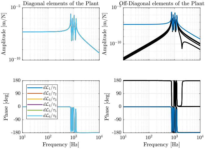
1.4 Plant Analysis
1.5 Controller Design
The controller consists of:
- A pure integrator
- A low pass filter with a cut-off frequency 3 times the crossover to increase the gain margin
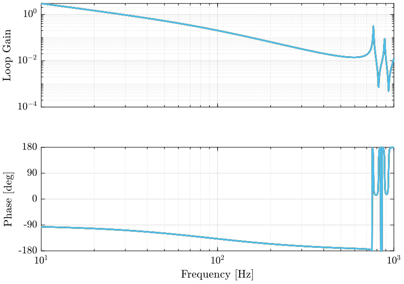
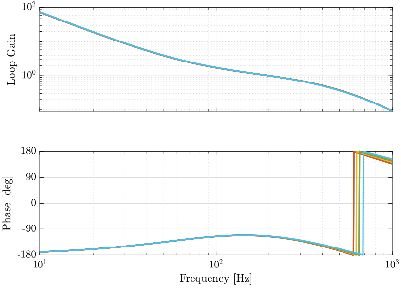
The obtained loop gains corresponding to the diagonal elements are shown in Figure 3.
wc = 2*pi*30;
Kl = diag(1./diag(abs(freqresp(G, wc)))) * wc/s * 1/(1 + s/3/wc);
1.6 Simulation
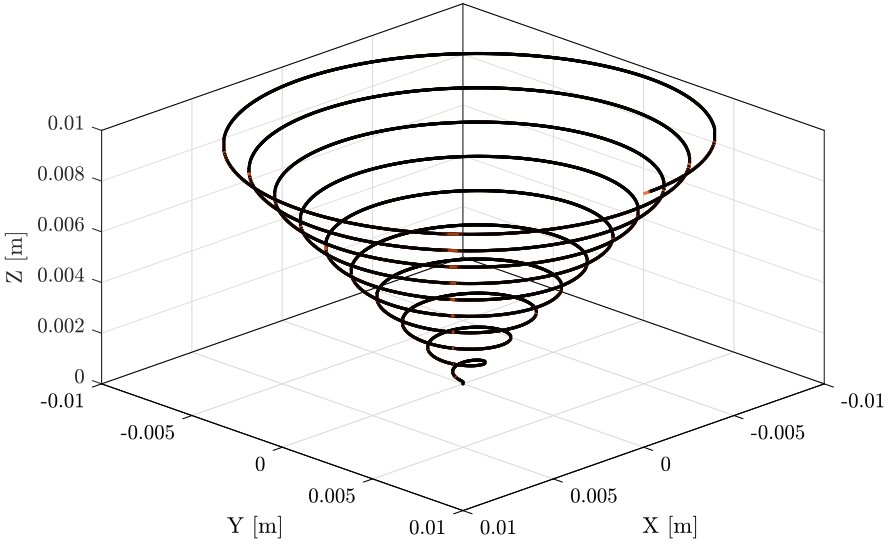
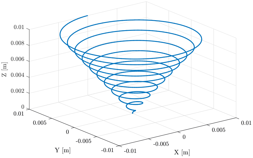
Let’s define some reference path to follow.
t = [0:1e-4:10];

r = zeros(6, length(t));

r(1, :) = 1e-3.*t.*sin(2*pi*t);
r(2, :) = 1e-3.*t.*cos(2*pi*t);
r(3, :) = 1e-3.*t;

references = initializeReferences(stewart, 't', t, 'r', r);
The reference path is shown in Figure 4.
figure;
plot3(squeeze(references.r.Data(1,1,:)), squeeze(references.r.Data(2,1,:)), squeeze(references.r.Data(3,1,:)));
xlabel('X [m]');
ylabel('Y [m]');
zlabel('Z [m]');
controller = initializeController('type', 'ref-track-L');
set_param('stewart_platform_model', 'StopTime', '10')
sim('stewart_platform_model');
simout_D = simout;
save('./mat/control_tracking.mat', 'simout_D', '-append');
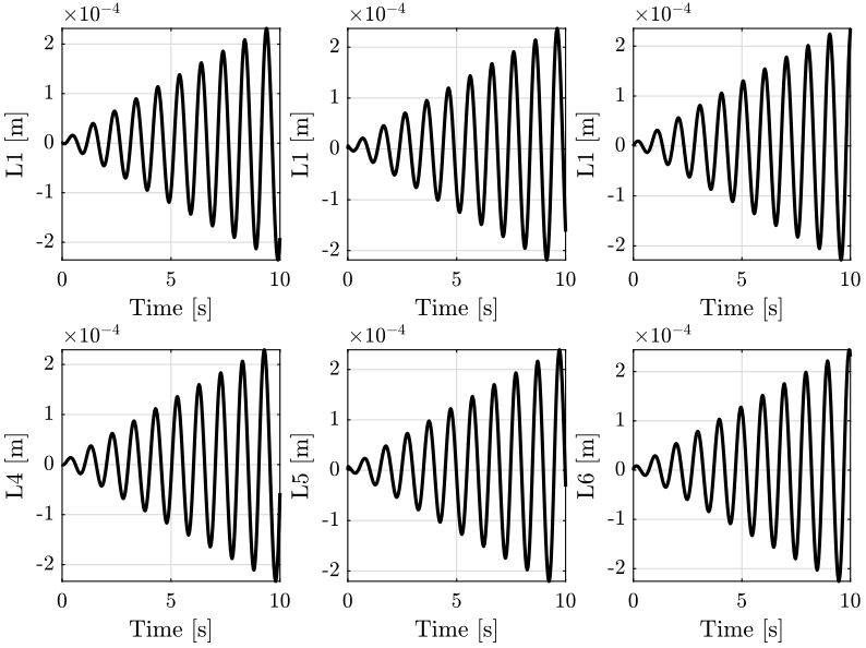
1.7 Results
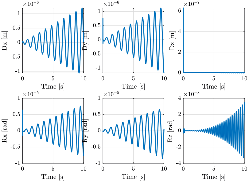
The reference path and the position of the mobile platform are shown in Figure 5.
figure;
hold on;
plot3(simout_D.x.Xr.Data(:, 1), simout_D.x.Xr.Data(:, 2), simout_D.x.Xr.Data(:, 3), 'k-');
plot3(squeeze(references.r.Data(1,1,:)), squeeze(references.r.Data(2,1,:)), squeeze(references.r.Data(3,1,:)), '--');
hold off;
xlabel('X [m]'); ylabel('Y [m]'); zlabel('Z [m]');
view([1,1,1])
zlim([0, inf]);
1.8 Conclusion
Such control architecture is easy to implement and give good results. The inverse kinematics is easy to compute.
However, as \(\mathcal{X}\) is not directly measured, it is possible that important positioning errors are due to finite stiffness of the joints and other imperfections.
2 Centralized Control Architecture using Pose Measurement
2.1 Control Schematic
The centralized controller takes the position error \(\bm{\epsilon}_\mathcal{X}\) as an inputs and generate actuator forces \(\bm{\tau}\) (see Figure 8). The signals are:
- reference path \(\bm{r}_\mathcal{X} = \begin{bmatrix} \epsilon_x & \epsilon_y & \epsilon_z & \epsilon_{R_x} & \epsilon_{R_y} & \epsilon_{R_z} \end{bmatrix}\)
- tracking error \(\bm{\epsilon}_\mathcal{X} = \begin{bmatrix} \epsilon_x & \epsilon_y & \epsilon_z & \epsilon_{R_x} & \epsilon_{R_y} & \epsilon_{R_z} \end{bmatrix}\)
- actuator forces \(\bm{\tau} = \begin{bmatrix} \tau_1 & \tau_2 & \tau_3 & \tau_4 & \tau_5 & \tau_6 \end{bmatrix}\)
- payload pose \(\bm{\mathcal{X}} = \begin{bmatrix} x & y & z & R_x & R_y & R_z \end{bmatrix}\)
![]()
Figure 8: Centralized Controller
Instead of designing a full MIMO controller \(K\), we first try to make the plant more diagonal by pre- or post-multiplying some constant matrix, then we design a diagonal controller.
We can think of two ways to make the plant more diagonal that are described in sections 2.4 and 2.5.
2.2 Initialize the Stewart platform
% Stewart Platform
stewart = initializeStewartPlatform();
stewart = initializeFramesPositions(stewart, 'H', 90e-3, 'MO_B', 45e-3);
stewart = generateGeneralConfiguration(stewart);
stewart = computeJointsPose(stewart);
stewart = initializeStrutDynamics(stewart);
stewart = initializeJointDynamics(stewart, 'type_F', 'universal_p', 'type_M', 'spherical_p');
stewart = initializeCylindricalPlatforms(stewart);
stewart = initializeCylindricalStruts(stewart);
stewart = computeJacobian(stewart);
stewart = initializeStewartPose(stewart);
stewart = initializeInertialSensor(stewart, 'type', 'accelerometer', 'freq', 5e3);

% Ground and Payload
ground = initializeGround('type', 'rigid');
payload = initializePayload('type', 'none');

% Controller
controller = initializeController('type', 'open-loop');

% Disturbances and References
disturbances = initializeDisturbances();
references = initializeReferences(stewart);
2.3 Identification of the plant
Let’s identify the transfer function from \(\bm{\tau}\) to \(\bm{\mathcal{X}}\).
%% Name of the Simulink File
mdl = 'stewart_platform_model';

%% Input/Output definition
clear io; io_i = 1;
io(io_i) = linio([mdl, '/Controller'],        1, 'openinput');  io_i = io_i + 1; % Actuator Force Inputs [N]
io(io_i) = linio([mdl, '/Relative Motion Sensor'],  1, 'openoutput'); io_i = io_i + 1; % Relative Displacement Outputs [m]

%% Run the linearization
G = linearize(mdl, io);
G.InputName  = {'F1', 'F2', 'F3', 'F4', 'F5', 'F6'};
G.OutputName = {'Dx', 'Dy', 'Dz', 'Rx', 'Ry', 'Rz'};
2.4 Diagonal Control - Leg’s Frame
2.4.1 Control Architecture
The pose error \(\bm{\epsilon}_\mathcal{X}\) is first converted in the frame of the leg by using the Jacobian matrix. Then a diagonal controller \(\bm{K}_\mathcal{L}\) is designed. The final implemented controller is \(\bm{K} = \bm{K}_\mathcal{L} \cdot \bm{J}\) as shown in Figure 9
Note here that the transformation from the pose error \(\bm{\epsilon}_\mathcal{X}\) to the leg’s length errors by using the Jacobian matrix is only valid for small errors.
![]()
Figure 9: Controller in the frame of the legs
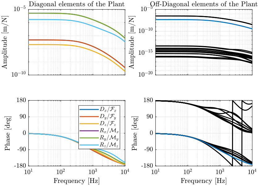
2.4.2 Plant Analysis
We now multiply the plant by the Jacobian matrix as shown in Figure 9 to obtain a more diagonal plant.
Gl = stewart.kinematics.J*G;
Gl.OutputName  = {'D1', 'D2', 'D3', 'D4', 'D5', 'D6'};
The bode plot of the plant is shown in Figure 10. We can see that the diagonal elements are identical. This will simplify the design of the controller as all the elements of the diagonal controller can be made identical.

We can see that this totally decouples the system at low frequency.
This was expected since: \[ \bm{G}(\omega = 0) = \frac{\delta\bm{\mathcal{X}}}{\delta\bm{\tau}}(\omega = 0) = \bm{J}^{-1} \frac{\delta\bm{\mathcal{L}}}{\delta\bm{\tau}}(\omega = 0) = \bm{J}^{-1} \text{diag}(\mathcal{K}_1^{-1} \ \dots \ \mathcal{K}_6^{-1}) \]
Thus \(J \cdot G(\omega = 0) = J \cdot \frac{\delta\bm{\mathcal{X}}}{\delta\bm{\tau}}(\omega = 0)\) is a diagonal matrix containing the inverse of the joint’s stiffness.
2.4.3 Controller Design
The controller consists of:
- A pure integrator
- A low pass filter with a cut-off frequency 3 times the crossover to increase the gain margin
The obtained loop gains corresponding to the diagonal elements are shown in Figure 11.
wc = 2*pi*30;
Kl = diag(1./diag(abs(freqresp(Gl, wc)))) * wc/s * 1/(1 + s/3/wc);

The controller \(\bm{K} = \bm{K}_\mathcal{L} \bm{J}\) is computed.
K = Kl*stewart.kinematics.J;
2.4.4 Simulation
We specify the reference path to follow.
t = [0:1e-4:10];

r = zeros(6, length(t));

r(1, :) = 1e-3.*t.*sin(2*pi*t);
r(2, :) = 1e-3.*t.*cos(2*pi*t);
r(3, :) = 1e-3.*t;

references = initializeReferences(stewart, 't', t, 'r', r);
controller = initializeController('type', 'ref-track-X');
We run the simulation and we save the results.
set_param('stewart_platform_model', 'StopTime', '10')
sim('stewart_platform_model')
simout_L = simout;
save('./mat/control_tracking.mat', 'simout_L', '-append');
2.5 Diagonal Control - Cartesian Frame
2.5.1 Control Architecture
A diagonal controller \(\bm{K}_\mathcal{X}\) take the pose error \(\bm{\epsilon}_\mathcal{X}\) and generate cartesian forces \(\bm{\mathcal{F}}\) that are then converted to actuators forces using the Jacobian as shown in Figure e 12.
The final implemented controller is \(\bm{K} = \bm{J}^{-T} \cdot \bm{K}_\mathcal{X}\).
![]()
Figure 12: Controller in the cartesian frame
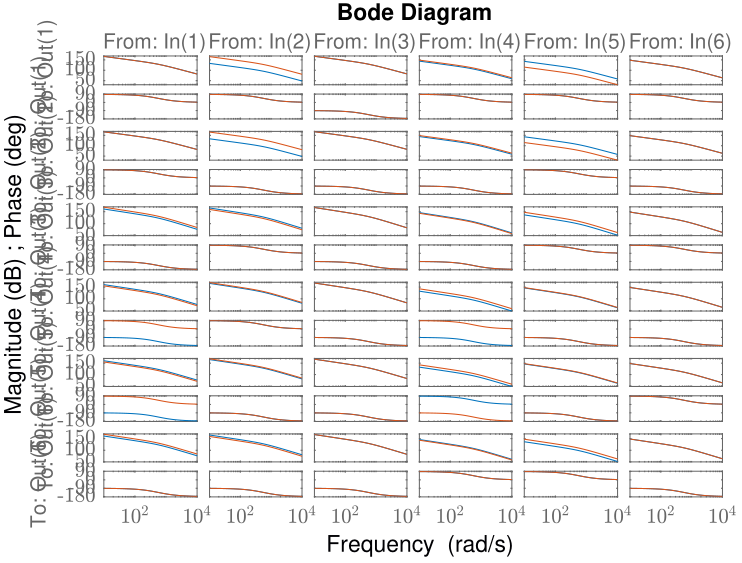
2.5.2 Plant Analysis
We now multiply the plant by the Jacobian matrix as shown in Figure 12 to obtain a more diagonal plant.
Gx = G*inv(stewart.kinematics.J');
Gx.InputName  = {'Fx', 'Fy', 'Fz', 'Mx', 'My', 'Mz'};
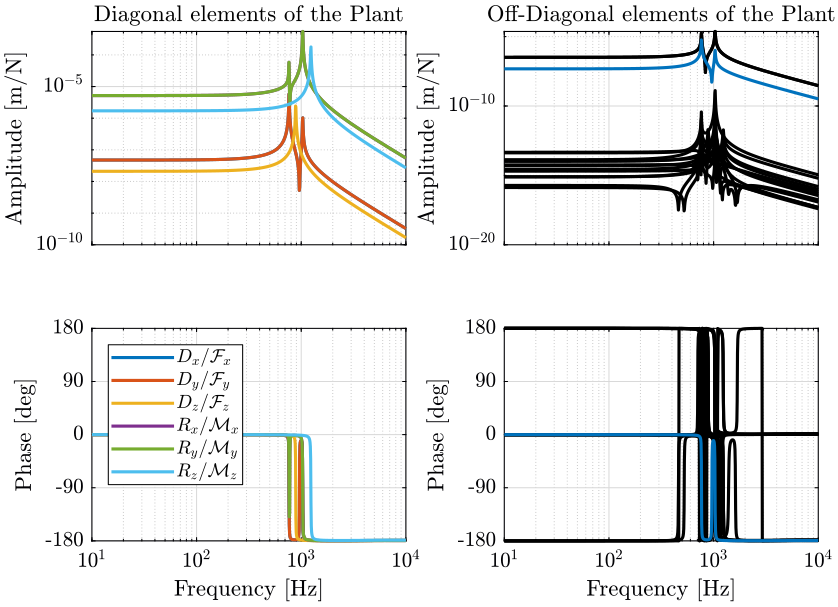
The diagonal terms are not the same. The resonances of the system are “decoupled”. For instance, the vertical resonance of the system is only present on the diagonal term corresponding to \(D_z/\mathcal{F}_z\).
Here the system is almost decoupled at all frequencies except for the transfer functions \(\frac{R_y}{\mathcal{F}_x}\) and \(\frac{R_x}{\mathcal{F}_y}\).
This is due to the fact that the compliance matrix of the Stewart platform is not diagonal.
| 4.75e-08 | -1.9751e-24 | 7.3536e-25 | 5.915e-23 | 3.2093e-07 | 5.8696e-24 |
| -7.1302e-25 | 4.75e-08 | 2.8866e-25 | -3.2093e-07 | -5.38e-24 | -3.2725e-23 |
| 7.9012e-26 | -6.3991e-25 | 2.099e-08 | 1.9073e-23 | 5.3384e-25 | -6.4867e-40 |
| 1.3724e-23 | -3.2093e-07 | 1.2799e-23 | 5.1863e-06 | 4.9412e-22 | -3.8269e-24 |
| 3.2093e-07 | 7.6013e-24 | 1.2239e-23 | 6.8886e-22 | 5.1863e-06 | -2.6025e-22 |
| 7.337e-24 | -3.2395e-23 | -1.571e-39 | 9.927e-23 | -3.2531e-22 | 1.7073e-06 |
One way to have this compliance matrix diagonal (and thus having a decoupled plant at DC) is to use a cubic architecture with the center of the cube’s coincident with frame \(\{A\}\).
This control architecture can also give a dynamically decoupled plant if the Center of mass of the payload is also coincident with frame \(\{A\}\).
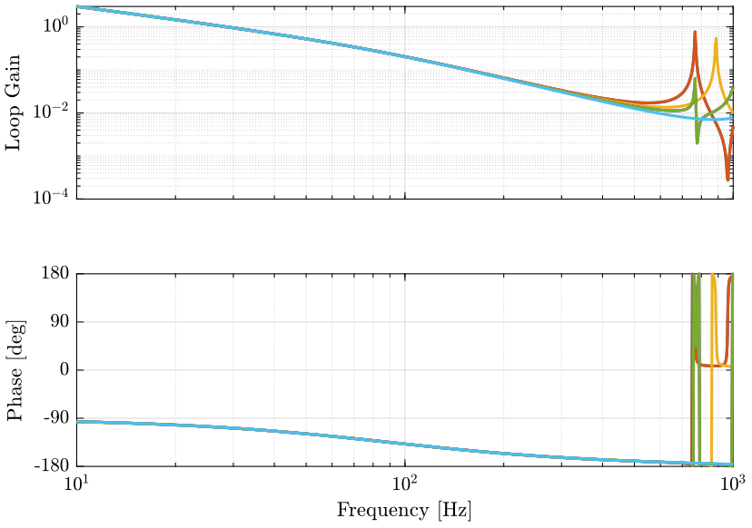
2.5.3 Controller Design
The controller consists of:
- A pure integrator
- A low pass filter with a cut-off frequency 3 times the crossover to increase the gain margin
The obtained loop gains corresponding to the diagonal elements are shown in Figure 14.
wc = 2*pi*30;
Kx = diag(1./diag(abs(freqresp(Gx, wc)))) * wc/s * 1/(1 + s/3/wc);
The controller \(\bm{K} = \bm{J}^{-T} \bm{K}_\mathcal{X}\) is computed.
K = inv(stewart.kinematics.J')*Kx;
2.5.4 Simulation
We specify the reference path to follow.
t = [0:1e-4:10];

r = zeros(6, length(t));

r(1, :) = 1e-3.*t.*sin(2*pi*t);
r(2, :) = 1e-3.*t.*cos(2*pi*t);
r(3, :) = 1e-3.*t;

references = initializeReferences(stewart, 't', t, 'r', r);
controller = initializeController('type', 'ref-track-X');
We run the simulation and we save the results.
set_param('stewart_platform_model', 'StopTime', '10')
sim('stewart_platform_model')
simout_X = simout;
save('./mat/control_tracking.mat', 'simout_X', '-append');
2.6 Diagonal Control - Steady State Decoupling
2.6.1 Control Architecture
The plant \(\bm{G}\) is pre-multiply by \(\bm{G}^{-1}(\omega = 0)\) such that the “shaped plant” \(\bm{G}_0 = \bm{G} \bm{G}^{-1}(\omega = 0)\) is diagonal at low frequency.
Then a diagonal controller \(\bm{K}_0\) is designed.
The control architecture is shown in Figure 15.
![]()
Figure 15: Static Decoupling of the Plant
2.6.2 Plant Analysis
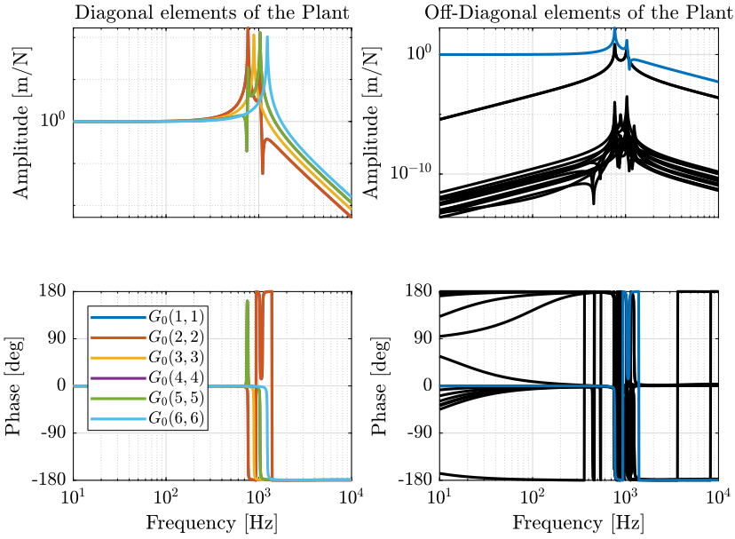
2.6.3 Controller Design
We have that: \[ \bm{G}^{-1}(\omega = 0) = \left(\frac{\delta\bm{\mathcal{X}}}{\delta\bm{\tau}}(\omega = 0)\right)^{-1} = \left( \bm{J}^{-1} \frac{\delta\bm{\mathcal{L}}}{\delta\bm{\tau}}(\omega = 0) \right)^{-1} = \text{diag}(\mathcal{K}_1^{-1} \ \dots \ \mathcal{K}_6^{-1}) \bm{J} \]
And because:
- all the leg stiffness are equal
- the controller equal to a \(\bm{K}_0(s) = k(s) \bm{I}_6\)
We have that \(\bm{K}_0(s)\) commutes with \(\bm{G}^{-1}(\omega = 0)\) and thus the overall controller \(\bm{K}\) is the same as the one obtain in section 2.4.
2.7 Comparison
2.7.1 Obtained MIMO Controllers
2.7.2 Simulation Results
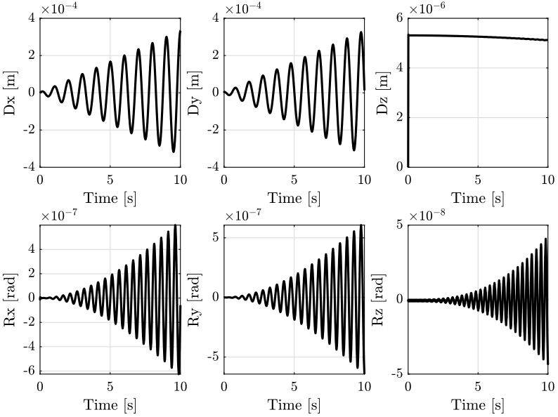
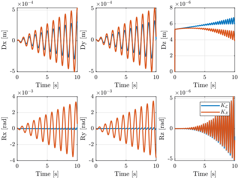
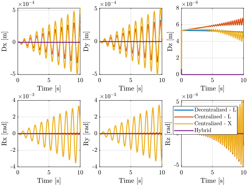
The position error \(\bm{\epsilon}_\mathcal{X}\) for both centralized architecture are shown in Figure 18.
Based on Figure 18, we can see that:
- There is some tracking error \(\epsilon_x\)
- The errors \(\epsilon_y\), \(\epsilon_{R_x}\) and \(\epsilon_{R_z}\) are quite negligible
- There is some error in the vertical position \(\epsilon_z\). The frequency of the error \(\epsilon_z\) is twice the frequency of the reference path \(r_x\).
- There is some error \(\epsilon_{R_y}\). This error is much lower when using the diagonal control in the frame of the leg instead of the cartesian frame.
2.8 Conclusion
Both control architecture gives similar results even tough the control in the Leg’s frame gives slightly better results.
The main differences between the control architectures used in sections 2.4 and 2.5 are summarized in Table 1.
| Leg’s Frame | Cartesian Frame | Static Decoupling | |
|---|---|---|---|
| Plant Meaning | \(\delta\mathcal{L}_i/\tau_i\) | \(\delta\mathcal{X}_i/\mathcal{F}_i\) | No physical meaning |
| Obtained Decoupling | Decoupled at DC | Dynamical decoupling except few terms | Decoupled at DC |
| Diagonal Elements | Identical with all the Resonances | Different, resonances are cancel out | No Alternating poles and zeros |
| Mechanical Architecture | Architecture Independent | Better with Cubic Architecture | |
| Robustness to Uncertainty | Good (only depends on \(J\)) | Good (only depends on \(J\)) | Bad (depends on the mass) |
These decoupling methods only uses the Jacobian matrix which only depends on the Stewart platform geometry. Thus, this method should be quite robust against parameter variation (e.g. the payload mass).
3 Hybrid Control Architecture - HAC-LAC with relative DVF
3.1 Control Schematic
Let’s consider the control schematic shown in Figure 19.
The first loop containing \(\bm{K}_\mathcal{L}\) is a Decentralized Direct (Relative) Velocity Feedback.
A reference \(\bm{r}_\mathcal{L}\) is computed using the inverse kinematics and corresponds to the wanted motion of each leg. The actual length of each leg \(\bm{\mathcal{L}}\) is subtracted and then passed trough the controller \(\bm{K}_\mathcal{L}\).
The controller is a diagonal controller with pure derivative action on the diagonal.
The effect of this loop is:
- it adds damping to the system (the force applied in each actuator is proportional to the relative velocity of the strut)
- it however does not go “against” the reference path \(\bm{r}_\mathcal{X}\) thanks to the use of the inverse kinematics
Then, the second loop containing \(\bm{K}_\mathcal{X}\) is designed based on the already damped plant (represented by the gray area). This second loop is responsible for the reference tracking.
![]()
Figure 19: Hybrid Control Architecture
3.2 Initialize the Stewart platform
% Stewart Platform
stewart = initializeStewartPlatform();
stewart = initializeFramesPositions(stewart, 'H', 90e-3, 'MO_B', 45e-3);
stewart = generateGeneralConfiguration(stewart);
stewart = computeJointsPose(stewart);
stewart = initializeStrutDynamics(stewart);
stewart = initializeJointDynamics(stewart, 'type_F', 'universal_p', 'type_M', 'spherical_p');
stewart = initializeCylindricalPlatforms(stewart);
stewart = initializeCylindricalStruts(stewart);
stewart = computeJacobian(stewart);
stewart = initializeStewartPose(stewart);
stewart = initializeInertialSensor(stewart, 'type', 'accelerometer', 'freq', 5e3);

% Ground and Payload
ground = initializeGround('type', 'rigid');
payload = initializePayload('type', 'none');

% Controller
controller = initializeController('type', 'open-loop');

% Disturbances and References
disturbances = initializeDisturbances();
references = initializeReferences(stewart);
3.3 First Control Loop - \(\bm{K}_\mathcal{L}\)
3.3.1 Identification
Let’s identify the transfer function from \(\bm{\tau}\) to \(\bm{L}\).
%% Name of the Simulink File
mdl = 'stewart_platform_model';

%% Input/Output definition
clear io; io_i = 1;
io(io_i) = linio([mdl, '/Controller'],        1, 'openinput');  io_i = io_i + 1; % Actuator Force Inputs [N]
io(io_i) = linio([mdl, '/Stewart Platform'],  1, 'openoutput', [], 'dLm'); io_i = io_i + 1; % Relative Displacement Outputs [m]

%% Run the linearization
Gl = linearize(mdl, io);
Gl.InputName  = {'F1', 'F2', 'F3', 'F4', 'F5', 'F6'};
Gl.OutputName = {'L1', 'L2', 'L3', 'L4', 'L5', 'L6'};
3.3.2 Obtained Plant

3.3.3 Controller Design
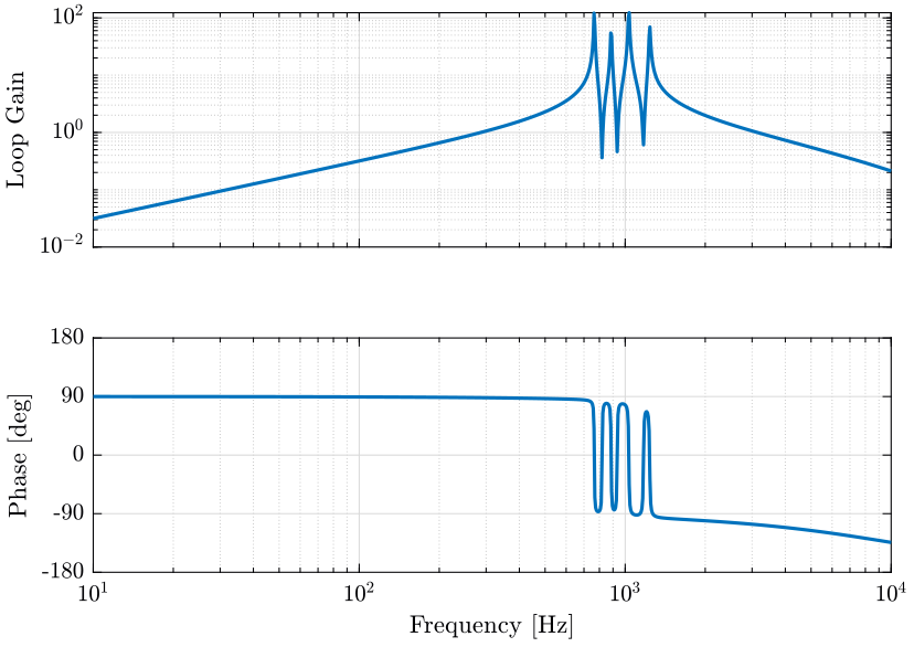
We apply a decentralized (diagonal) direct velocity feedback. Thus, we apply a pure derivative action. In order to make the controller realizable, we add a low pass filter at high frequency. The gain of the controller is chosen such that the resonances are critically damped.
The obtain loop gain is shown in Figure 21.
Kl = 1e4 * s / (1 + s/2/pi/1e4) * eye(6);
3.4 Second Control Loop - \(\bm{K}_\mathcal{X}\)
3.4.1 Identification
Kx = tf(zeros(6));

controller = initializeController('type', 'ref-track-hac-dvf');
%% Name of the Simulink File
mdl = 'stewart_platform_model';

%% Input/Output definition
clear io; io_i = 1;
io(io_i) = linio([mdl, '/Controller'],              1, 'input');  io_i = io_i + 1; % Actuator Force Inputs [N]
io(io_i) = linio([mdl, '/Relative Motion Sensor'],  1, 'openoutput'); io_i = io_i + 1; % Relative Displacement Outputs [m]

%% Run the linearization
G = linearize(mdl, io);
G.InputName  = {'F1', 'F2', 'F3', 'F4', 'F5', 'F6'};
G.OutputName = {'Dx', 'Dy', 'Dz', 'Rx', 'Ry', 'Rz'};
3.4.2 Obtained Plant
We use the Jacobian matrix to apply forces in the cartesian frame.
Gx = G*inv(stewart.kinematics.J');
Gx.InputName  = {'Fx', 'Fy', 'Fz', 'Mx', 'My', 'Mz'};
The obtained plant is shown in Figure 22.
3.4.3 Controller Design
The controller consists of:
- A pure integrator
- A Second integrator up to half the wanted bandwidth
- A Lead around the cross-over frequency
- A low pass filter with a cut-off equal to three times the wanted bandwidth
wc = 2*pi*200; % Bandwidth Bandwidth [rad/s]

h = 3; % Lead parameter

Kx = (1/h) * (1 + s/wc*h)/(1 + s/wc/h) * wc/s * ((s/wc*2 + 1)/(s/wc*2)) * (1/(1 + s/wc/3));

% Normalization of the gain of have a loop gain of 1 at frequency wc
Kx = Kx.*diag(1./diag(abs(freqresp(Gx*Kx, wc))));
Then we include the Jacobian in the controller matrix.
Kx = inv(stewart.kinematics.J')*Kx;
3.5 Simulations
We specify the reference path to follow.
t = [0:1e-4:10];

r = zeros(6, length(t));

r(1, :) = 1e-3.*t.*sin(2*pi*t);
r(2, :) = 1e-3.*t.*cos(2*pi*t);
r(3, :) = 1e-3.*t;

references = initializeReferences(stewart, 't', t, 'r', r);
We run the simulation and we save the results.
set_param('stewart_platform_model', 'StopTime', '10')
sim('stewart_platform_model')
simout_H = simout;
save('./mat/control_tracking.mat', 'simout_H', '-append');
The obtained position error is shown in Figure 24.
3.6 Conclusion
4 Comparison of all the methods
5 Compute the pose error of the Stewart Platform
Let’s note:
- \(\{W\}\) the fixed measurement frame (corresponding to the metrology frame / the frame where the wanted displacement are expressed). The center of the frame if \(O_W\)
- \(\{M\}\) is the frame fixed to the measured elements. \(O_M\) is the point where the pose of the element is measured
- \(\{R\}\) is a virtual frame corresponding to the wanted pose of the element. \(O_R\) is the origin of this frame where the we want to position the point \(O_M\) of the element.
- \(\{V\}\) is a frame which its axes are aligned with \(\{W\}\) and its origin \(O_V\) is coincident with the \(O_M\)
Reference Position with respect to fixed frame {W}: \({}^WT_R\)
Dxr = 0;
Dyr = 0;
Dzr = 0.1;
Rxr = pi;
Ryr = 0;
Rzr = 0;
Measured Position with respect to fixed frame {W}: \({}^WT_M\)
Dxm = 0;
Dym = 0;
Dzm = 0;
Rxm = pi;
Rym = 0;
Rzm = 0;
We measure the position and orientation (pose) of the element represented by the frame \(\{M\}\) with respect to frame \(\{W\}\). Thus we can compute the Homogeneous transformation matrix \({}^WT_M\).
%% Measured Pose
WTm = zeros(4,4);

WTm(1:3, 1:3) = [cos(Rzm) -sin(Rzm) 0;
     sin(Rzm)  cos(Rzm) 0;
     0        0         1] * ...
    [cos(Rym)  0        sin(Rym);
     0        1        0;
     -sin(Rym)  0        cos(Rym)] * ...
    [1        0        0;
     0        cos(Rxm) -sin(Rxm);
     0        sin(Rxm)  cos(Rxm)];
WTm(1:4, 4) = [Dxm ; Dym ; Dzm; 1];
We can also compute the Homogeneous transformation matrix \({}^WT_R\) corresponding to the transformation required to go from fixed frame \(\{W\}\) to the wanted frame \(\{R\}\).
%% Reference Pose
WTr = zeros(4,4);

WTr(1:3, 1:3) = [cos(Rzr) -sin(Rzr) 0;
     sin(Rzr)  cos(Rzr) 0;
     0        0         1] * ...
    [cos(Ryr)  0        sin(Ryr);
     0        1        0;
     -sin(Ryr)  0        cos(Ryr)] * ...
    [1        0        0;
     0        cos(Rxr) -sin(Rxr);
     0        sin(Rxr)  cos(Rxr)];
WTr(1:4, 4) = [Dxr ; Dyr ; Dzr; 1];
We can also compute \({}^WT_V\).
WTv = eye(4);
WTv(1:3, 4) = WTm(1:3, 4);
Now we want to express \({}^MT_R\) which corresponds to the transformation required to go to wanted position expressed in the frame of the measured element. This homogeneous transformation can be computed from the previously computed matrices: \[ {}^MT_R = ({{}^WT_M}^{-1}) {}^WT_R \]
%% Wanted pose expressed in a frame corresponding to the actual measured pose
MTr = [WTm(1:3,1:3)', -WTm(1:3,1:3)'*WTm(1:3,4) ; 0 0 0 1]*WTr;
Now we want to express \({}^VT_R\): \[ {}^VT_R = ({{}^WT_V}^{-1}) {}^WT_R \]
%% Wanted pose expressed in a frame coincident with the actual position but with no rotation
VTr = [WTv(1:3,1:3)', -WTv(1:3,1:3)'*WTv(1:3,4) ; 0 0 0 1] * WTr;
%% Extract Translations and Rotations from the Homogeneous Matrix
T = MTr;
Edx = T(1, 4);
Edy = T(2, 4);
Edz = T(3, 4);

% The angles obtained are u-v-w Euler angles (rotations in the moving frame)
Ery = atan2( T(1, 3),          sqrt(T(1, 1)^2 + T(1, 2)^2));
Erx = atan2(-T(2, 3)/cos(Ery), T(3, 3)/cos(Ery));
Erz = atan2(-T(1, 2)/cos(Ery), T(1, 1)/cos(Ery));